---
title: "Chapt 0: Starter"
navbar: false
language:
en:
title-block-author-single: "Author"
title-block-published: "Updated"
zh:
title-block-author-single: "作者"
title-block-published: "更新时间"
author:
- name: "Feng Wan"
email: wanfeng@xjtu.edu.cn
orcid: 0000-0002-9715-3032
affiliations:
- name: "B832@仲英楼 or 3133@泓理楼 // School of Physcis @ Xian Jiaoton University"
address: "B832@仲英楼 or 3133@泓理楼"
---
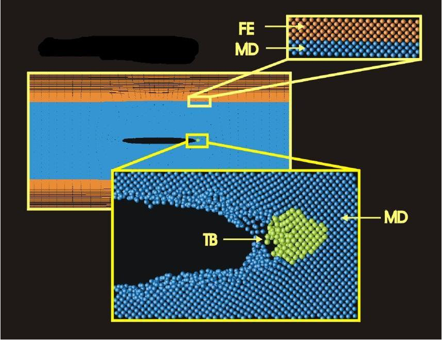
## Molecule dynamics
### Laser induced MD
::: {#fig-Laser-induced-MD layout-ncol=2}
{group="my-gallery"}
{group="my-gallery"}
激光脉冲引起的二苯乙烯分子的异构化反应的分子动力学模拟结果
:::
---
"){fig-align="center"}
------------------------------------------------------------------------
### Silicon crystal defects
{fig-align="center"}
> Modeling materials on different length scales:
>
> - quantum mechanics (tight binding)
>
> - classical forces (molecular dynamics)
>
> - continuum mechanics (finite element)
------------------------------------------------------------------------
### Neutron shelding via Monte Carlo
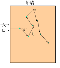{fig-align="center"}
- 模型的建立\
假设铅墙厚度为5,中子在铅中的平均自由程为1,中子与铅原子碰撞后各向同性散射。令碰撞*8次*后中子能量耗尽
- 中子的水平位移$S$为\
$1+ \cos\theta_1 + \cos\theta_2 +\cos\theta_3 +\cos\theta_4 +\cos\theta_5 +\cos\theta_6 +\cos\theta_7 +\cos\theta_8$
- 当中子的水平位移$S$大于5时,中子则穿透了铅墙;小于0时,则表明中子反射回来了;位移S的值在0到5之间时,则表示中子被铅墙吸收了。
------------------------------------------------------------------------
``` {.matlab filename="neutron.m"}
clear all
close all
clc
format long

    N=50000;
    x1=rand(1,N)*2*pi; %注意随机数要在计算函数值和误差,方差前给定
    x2=rand(1,N)*2*pi;
    x3=rand(1,N)*2*pi;
    x4=rand(1,N)*2*pi;
    x5=rand(1,N)*2*pi;
    x6=rand(1,N)*2*pi;
    x7=rand(1,N)*2*pi;
    s=1+cos(x1)+cos(x2)+cos(x3)+cos(x4)+cos(x5)+cos(x6)+cos(x7);

    N_1=0;
    N_2=0;
    N_3=0;
for i=1:N
    if s(i)<0      %计算被隔离墙反射的中子数目
        N_1=N_1+1;
    elseif s(i)>5
        N_2=N_2+1; %计算穿过隔离墙的中子数目
    else
        N_3=N_3+1; %计算被隔离墙吸收的中子数目
    end
end
N_1/N
N_2/N  %计算穿过隔离墙的中子的比例
N_3/N
%figure;plot(1:N,x1/2/pi,'*')
%figure;plot(1:N,s,'*')
figure('Position', [100 100 1000 400]);
subplot(121)
histogram(s, 100);
set(gca, 'fontsize', 18, 'linewidth', 1.5)
subplot(122)
[cy, cx] = histcounts(s, 100);
plot(cx(2:end), cy / N, 'k-', 'linewidth', 3);
hold on;
plot(cx(2:end), smooth(cy / N), 'r-', 'linewidth', 3);
set(gca, 'fontsize', 18, 'linewidth', 1.5)
```
------------------------------------------------------------------------
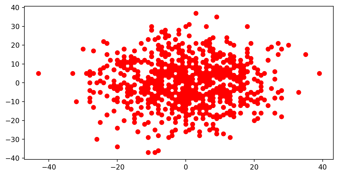
### Random walk (MC)
蒙特卡罗方法应用实例:随机行走问题
> 一醉汉从原点随机选择(上,下,左,右)方向开始移动,经过N步移动后(每步移动的距离为1),求距原点的距离
``` {.matlab filename="random-walk.m"}
clear all
close all
clc

N = 300;    % 每次行走步数为 N。
number=800;

step = [[1,0]; [-1, 0]; [0, 1]; [0, -1]];   % 可选的四种不同的位移矢量

for j=1:number
    zuobiao = [0, 0];       % 初始位置为原点
    for i = 1:N             % 行走 N 步
        k = ceil(4*rand()); % 随机选择方向 1、2、3、4,注意,ceil(x) 函数返回不小于 x 的最小整数,如 ceal(0.4)= 1.
        zuobiao = zuobiao + step(k,:);   %更新坐标,即在上一步坐标上加上位移矢量。
        %plot(0,0,'ro',zuobiao(1),zuobiao(2),'*')
    end
    hold on
    plot(0,0,'ro',zuobiao(1),zuobiao(2),'*')
end
   % r = norm(zuobiao)
```
------------------------------------------------------------------------
```{python}
import numpy as np
import matplotlib.pyplot as plt
N = 300
number = 800
step = np.reshape(np.array([1, 0, -1, 0, 0, 1, 0, -1]), [4, 2])
for i in range(number):
    position = np.array([0, 0])
    for j in range(N):
        k = np.floor(4.0 * np.random.rand())
        position = position + step[np.int64(k)]
    plt.plot(position[0], position[1], 'ro')
plt.show()
```
## simulation examples
### Black hole accretion
{{< video videos/nasa-blackhole.mp4 title="black hole simulation" >}}
### Proton-Proton scattering
{{< video videos/proton-proton.mp4 title="proton proton scattering" >}}
### Helmholtz instability
{{< video videos/instability.mp4 title="fluid instability" >}}
### Wakefield acceleration
{{< video videos/wakefield.mp4 title="wakefield acceleration" >}}
### Quantum scattering
{{< video videos/quantum-scattering.mp4 title="quantum wavepacket scattering" >}}
See more: [https://github.com/quantum-visualizations/qmsolve.git](https://github.com/quantum-visualizations/qmsolve.git)
How to run the code:
1. ``` pip install qmsolve ```
2. ``` python examples/xxx.py ```
### Ising model
{{< video videos/ising-model.mp4 title="Ising model" >}}
See more: [http://mattbierbaum.github.io/ising.js/](http://mattbierbaum.github.io/ising.js/)
## Computational Physcis
以计算机及计算机技术为工具和手段,运用计算科学所提供的各种方法,解决复杂的物理问题的一门应用科学 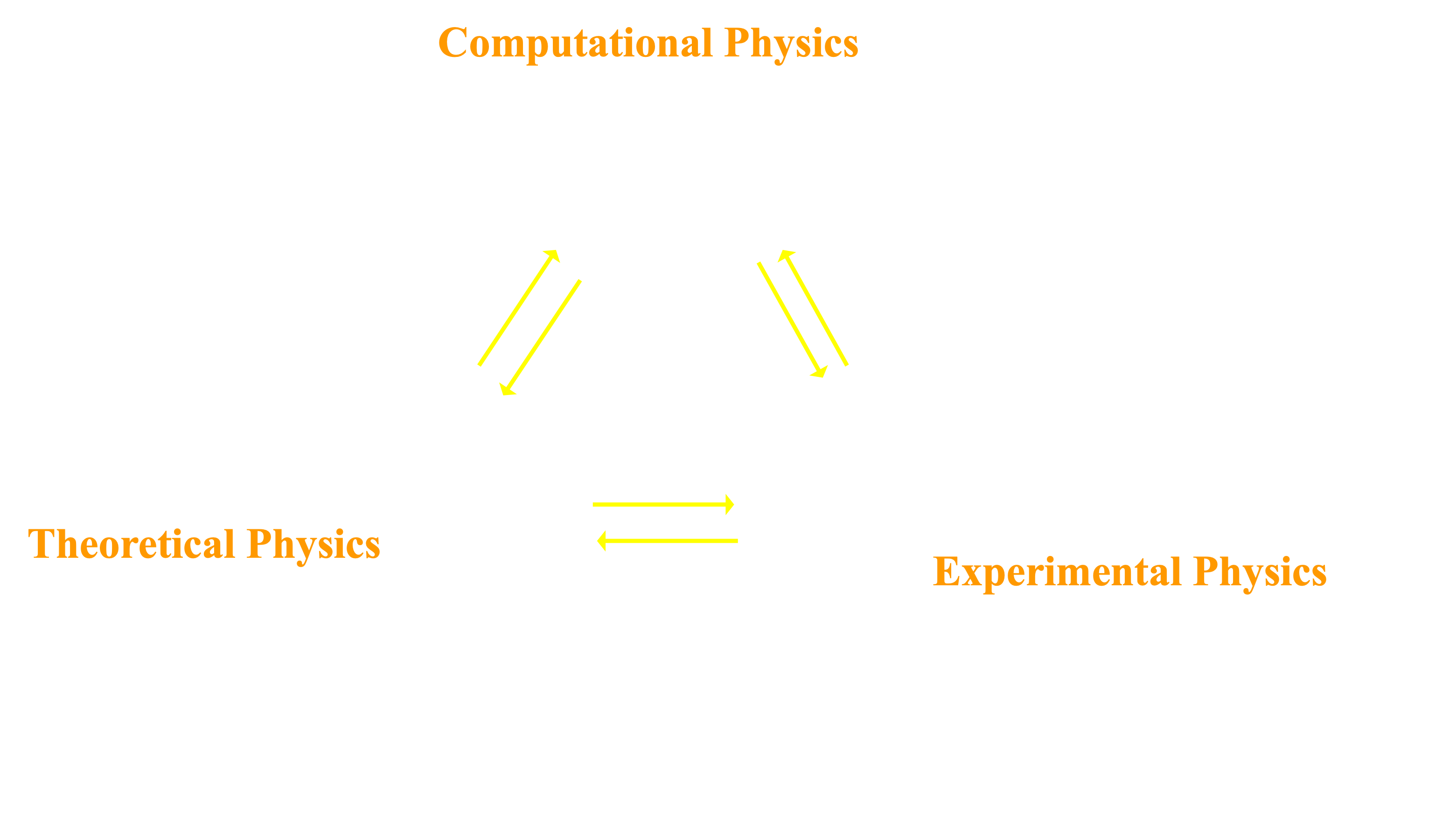
## History & Fate of ***ComPhys***
### History
- 20世纪40年代初,二战时期核武器研制中涉及的复杂问题,使得计算机介入物理学的研究在所难免
- 计算机的飞速发展
- 为报导计算物理领域的研究成果,召开学术会议、出版发行学术期刊
- 1963年 Livermore实验室的Berni & Alder编辑出版 Methods in Computational physics
- 1966年 美国的 Berni & Alder 主编创刊 Journal of Computational physics\
- 1969年 英国的 Burki 主编在西欧创刊 Computer physics Communication
- 1984年9月中国出版《计算物理》杂志
---
### Contents and methods
- Programming language
- Algorithms
- Program design
- Computer solving
::: {.callout-note icon=false}
采用计算科学的方法,应用大规模高速计算机作为工具,解决理论或实验物理范畴的极其复杂的问题。
:::
+ TheoPhys ...
+ ExpPhys ...
---
(@) 研究首要问题是建立起相应的物理、数学模型,选择算法并使之可在计算机上实现 $$I(x) = \int_a^b \exp\left(-x^2\right)dx$$ $$\frac{2}{\pi}\int_1^\infty e^{-\xi^2}d\xi = 0.1573$$
(@) 第二个问题是算法的误差问题
- 模型误差 —— 次要因素的忽略、各种限制等
- 观测误差 —— 模型中常包含一些通过实验测量而获得的物理参数。 如:比重、比热等等
- 方法误差 —— 数学模型一般相当复杂,不能获得其精确解,或有些运算只能用极限过程定义,而计算机 只能进行有限次运算(截断误差)
$$e^x = \sum_{n=0}^\infty \frac{x^n}{n!} ~~~ S_n(x) = \sum_{i=0}^\infty \frac{x^i}{i!}$$
$$ R_n(x) = \frac{x^{n+1}}{(n+1)!}e^{\theta x}~~ 0<\theta<1$$
- 舍入误差 —— 计算机的有限字长(计算误差)
(@) 最后一个问题是计算的收敛性和稳定性问题
::: {.callout-caution}
收敛性主要研究算法误差的变化问题,而稳定性则更关注于舍入误差的问题
- 如何评价一个算法的好坏
- 计算结果的精度,即误差大小
- 得到结果需要付出的代价 -- 时空复杂性
:::
---
## References
* 主要参考教材:《计算物理学》 [美] Steven E.Koonin 著 秦克诚 译 高等教育出版社
* 参考书:
+ 《计算物理学》,顾昌鑫,复旦大学出版社
+ 《An Introduction to Computational Physics》,Tao Pang, Cambridge University Press
+ 《精通Matlab R2011a》, 张志涌,北京航空航天大学出版社。
+ 《计算机模拟方法在物理学中的应用》,Harvey Gould等,高等育出版社
+ 《计算物理基础》,彭芳麟,高等教育出版社
## Course Information
+ 教师:弯峰 赵前 徐忠锋 栗建兴
+ 助教:{{< var zhujiao.name >}} 负责《思源学习空间》课程资源建设与维护
+ contacts:
- 弯 峰: 157 7191 0192
- 赵 前: 189 3031 8061
- 徐忠锋: 133 0929 8803
- 栗建兴: 151 2927 3796
- {{< var zhujiao.name >}}: {{< var zhujiao.phone >}}
+ tasks:
- 课堂布置:算法巩固与应用
- 算例:3/5(5个任选2个,第十周上课前向老师报备)
---
### Others
- website: {{< var online.website >}}
- QQ group: {{< var online.qq >}}
{fig-align="center" width="600"}
## Evaluation
| Categories | Ratio | Remarks |
|---------|:-----|------:|
| Exercise | 20% | Homework |
| Regular performance | 10% | course |
| Seminar | 20% | 2/5 |
| Thesis | 50% | Free |
::: {.callout-note icon=false}
+ Homework — 以常用算法训练为主
+ Seminar — 每位同学1次课堂算例展示
+ Thesis — 每算例/大作业最多可3人合作,老师首先评定算例/大作业得分,即首位得分,排第2减5分,第三减10分;也可根据同学们提交时同时按分工任务设定3人的比例。
- 如某算例/大作业得分90分,3人得分分别为:方法一 90/85/80;方法二(假设比例为4:3:3)100/76.5/76.5
:::
## Course Plan
| Chapter | Content | Course hours | Extra |
|-------|:-------|:--------:|-------:|
| 0 | Starter | 2 | |
| 1 | Diff, Integral & Roots | 5 | |
| 2 | IVP of ODE | 5 | |
| 3 | BVP & EVP of ODE | 6 | |
| 4 | PDE (Elliptic, Parabolic & Heli) | 6 | |
| 5 | Monte Carlo | 6 | |
| 6 | Molecule Dynamics | 4 | |
::: {.callout-important appearance='simple'}
## Topics in seminar:
- vibration energy level of two atoms molecule system
- orders and chaos in dynamics
- 1D schodinger equation
- 1D t-d schodinger equation
- 2D Ising model
:::
::: {#exr-Python}
Use python write a simple code to print the Fibonacci series.
:::
::: {#sol-}
```{python}
print("hello world")
```
:::


")