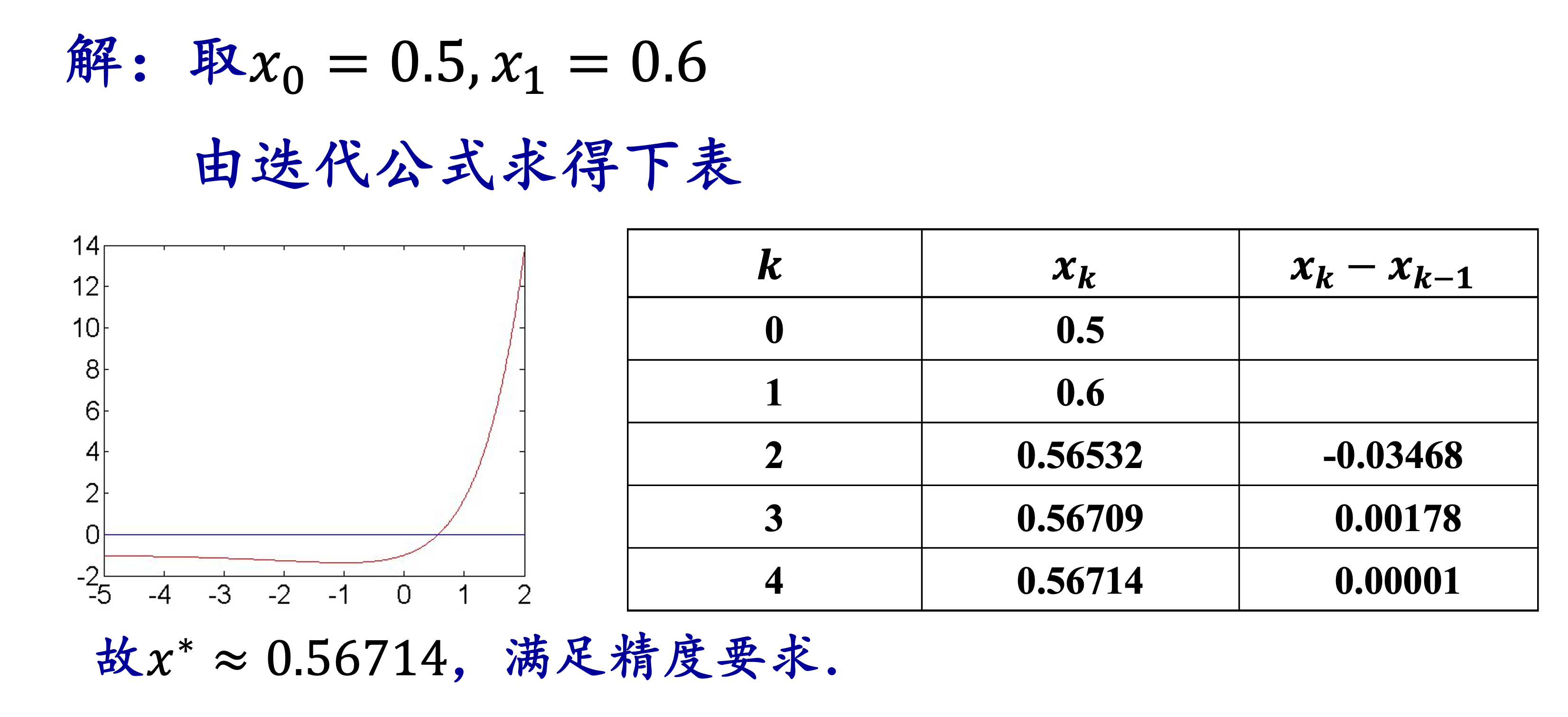
take \(k = 0, x_1 =\simeq x_0 - \frac{f(x_0)}{f'(x_0)}\)
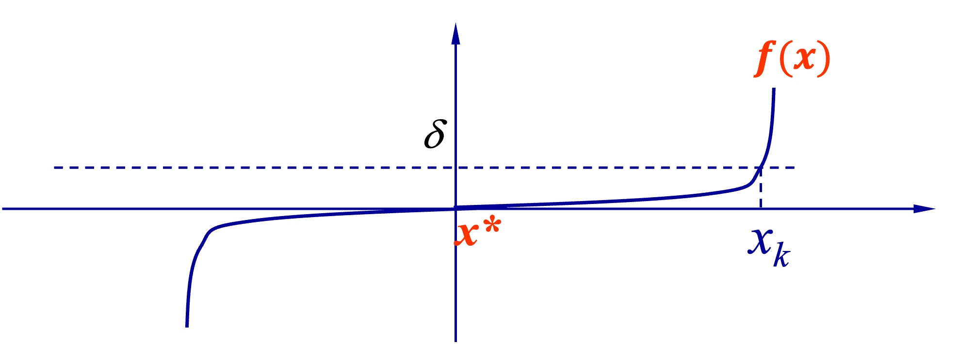
只用\(|f(x)|<\delta\)可能造成误差偏大
只用\(x_{k+1}-x_k < \varepsilon_1\)可能造成误差偏大
Newton iteration
%%{ init : { "theme" : "neutral", "flowchart" : { "curve" : "linear" }}}%%

graph LR

A["`init x(0), error d, e;
k = 0`"]
B["x(k+1) = x(k) - f(k) / f'(k)"]
C{"`|f(k)| < d and
|x(k+1) - x(k)| < e`"}
D["k = k + 1"]
E["stop"]
A --> B --> C --> |true| E
C --> |false| D --> B
%%{ init : { "theme" : "neutral", "flowchart" : { "curve" : "linear" }}}%%

graph LR

A("`init x(0), x(1), error d, e;
k = 0`")
C["Core"]
B{"`|f(k)| < d and
|x(k+1) - x(k)| < e`"}
D["k = k + 1"]
E["stop"]
A --> B --> |true| E
B --> |false| C --> D --> B
#!/usr/bin/env python"""Implements a variety of root-finding methods, including providing estimatesof convergence rates.USAGE: (from shell prompt) python ./findroot.pyAUTHOR: Jonathan Senning <jonathan.senning@gordon.edu> Gordon College Python Version: March 8, 2008"""import math#------------------------------------------------------------------------------def bisect( f, a, b, tol, maxiter ):""" Usage: ( x, rate ) = bisect( f, a, b, tol, maxiter ) This function uses bisection to solve f(x) = 0. This function requires that the function f(x) be already defined, and that its name be passed in as a string as the first argument. """def sign( x ):if x <0:return-1elif x >0:return1else:return0 x = a fa = f( a ) fb = f( b )# Make sure that (according to the Intermediate Value Theorem) the# specified interval does contain a root.if sign( fa ) == sign( fb ):print ("Interval [%f,%f] may not contain a root"% ( a, b ))# Initialize for the search. Note that we try and minimize the number# of evaluations of f(x). It is initially evaluated twice before the# iteration begins and then once during each iteration. These extra# points are needed to start off the error calculation which compares# estimates of solutions just computed with previous estimates. x0 = x +4.0* tol x1 = x +8.0* tol k =0while k <= maxiter: x2, x1, x0 = ( x1, x0, x ) x = ( a + b ) /2.0 fx = f( x ) max_error =abs( b - a ) /2.0print ("%2d%18.11e%18.11e%18.11e%18.11e"% ( k, a, b, x, max_error )) k = k +1if max_error < tol:breakif sign( fa ) == sign( fx ): a, fa = ( x, fx )else: b = xif k > maxiter:print ("Error: exceeded %d iterations"% maxiter) rate = math.log( abs((x - x0) / (x0 - x1)) ) /\ math.log( abs((x0 - x1) / (x1 - x2)) )return ( x, rate )#------------------------------------------------------------------------------def newton( f, df, x, tol, maxiter ):""" Usage: ( x, rate ) = newton( f, df, x, tol, maxiter ) This function performs a Newton-Raphson iteration to solve f(x) = 0. This function requires that the functions f(x) and df(x) (the first derivative of f with respect to x) both be already defined, and that their names be passed in as a strings as the first two arguments. """ x1 = x +8.0* tol x0 = x +4.0* tol k =0while k <= maxiter andabs( x - x0 ) >= tol: x2, x1, x0 = ( x1, x0, x ) x = x - f( x ) / df( x )print ("%2d%18.11e%18.11e"% ( k, x, abs( x - x0 ) )) k = k +1if k > maxiter:print ("Error: exceeded %d iterations"% maxiter) rate = math.log( abs((x - x0) / (x0 - x1)) ) /\ math.log( abs((x0 - x1) / (x1 - x2)) )return ( x, rate )#------------------------------------------------------------------------------def secant( f, x, tol, maxiter ):""" Usage: ( x, rate ) = secant( f, x, tol, maxiter ) This function performs a secant iteration to solve f(x) = 0. This function requires that the function f(x) be already defined, and that its name be passed in as a string as the first argument. """# These extra points are needed to start off the error calculation which# compares estimates of solutions just computed with previous estimates. x1 = x +8.0* tol x0 = x +4.0* tol fx0 = f(x0 ) k =0while k <= maxiter andabs( x - x0 ) >= tol: x2, x1, x0, fx1 = ( x1, x0, x, fx0 ) fx0 = f( x0 ) x = x0 - fx0 * ( x0 - x1 ) / ( fx0 - fx1 )print ("%2d%18.11e%18.11e"% ( k, x, abs( x - x0 ) )) k = k +1if k > maxiter:print ("Error: exceeded %d iterations"% maxiter) rate = math.log( abs((x - x0) / (x0 - x1)) ) /\ math.log( abs((x0 - x1) / (x1 - x2)) )return ( x, rate )#------------------------------------------------------------------------------def fixedpoint( f, x, a, tol, maxiter ):""" Usage: ( x, rate ) = fixedpoint( f, x, a, tol, maxiter ) This function performs a fixed point iteration to solve f(x) = 0. It constructs a function g(x) = x + a * f(x) so that p = g(p) when f(p) = 0. The value of "a" is choosen to speed convergence -- it should make g'(p) = 0 where p is the solution of f(p) = 0. This function requires that the function f(x) be already defined, and that its name be passed in as a string as the first argument. """# These extra points are needed to start off the error calculation which# compares estimates of solutions just computed with previous estimates. x1 = x +8.0* tol x0 = x +4.0* tol k =0while k <= maxiter andabs( x - x0 ) >= tol: x2, x1, x0 = ( x1, x0, x ) x = x + a * f( x )print ("%2d%18.11e%18.11e"% ( k, x, abs( x - x0 ) )) k = k +1if k > maxiter:print ("Error: exceeded %d iterations"% maxiter) rate = math.log( abs((x - x0) / (x0 - x1)) ) /\ math.log( abs((x0 - x1) / (x1 - x2)) )return ( x, rate )#------------------------------------------------------------------------------def steffensen( f, x, a, tol, maxiter ):""" Usage: ( x, rate ) = steffensen( f, x, a, tol, maxiter ) This function performs a steffensen's iteration to solve f(x) = 0. It constructs a function g(x) = x + a * f(x) so that p = g(p) when f(p) = 0. The value of "a" is choosen to speed convergence -- it should make g'(p) = 0 where p is the solution of f(p) = 0. This function requires that the function f(x) be already defined, and that its name be passed in as a string as the first argument. """# These extra points are needed to start off the error calculation which# compares estimates of solutions just computed with previous estimates. x1 = x +8.0* tol x0 = x +4.0* tol k =0while k <= maxiter andabs( x - x0 ) >= tol: x2, x1, x0 = ( x1, x0, x ) p1 = x + a * f( x ) p2 = p1 + a * f( p1 ) x = x - ( ( p1 - x )**2 ) / ( p2 -2* p1 + x )print ("%2d%18.11e%18.11e"% ( k, x, abs( x - x0 ) )) k = k +1if k > maxiter:print ("Error: exceeded %d iterations"% maxiter) rate = math.log( abs((x - x0) / (x0 - x1)) ) /\ math.log( abs((x0 - x1) / (x1 - x2)) )return ( x, rate )#------------------------------------------------------------------------------#------------------------------------------------------------------------------#------------------------------------------------------------------------------if__name__=="__main__":""" J. R. Senning <jonathan.senning@gordon.edu> Gordon College Python Version: March 8, 2008 This program uses five different root-finding algorithms to solve f(x) = 0. """# Maximum number of iterations maxiter =100# Tolerance for all algorithms. This value determines how accurate# the final estimate of the root will be. tol =1e-8# ---------- Define f(x), df(x) and the interval to search -------------def f(x): return1- x * math.exp( x )def df(x): return-( 1+ x ) * math.exp( x ) a, b = ( 0.0, 2.0 ) first_guess = ( a + b ) /2.0print ("************************************************************")print ("Finding root of f(x) = 1 - x * exp(x) on [%f,%f]"% ( a, b ))print ("************************************************************")# ======================================================================# ---------- Bisection Method ------------------------------------------# ======================================================================print ("\n-------- Bisection Method ---------------------------\n") x, rate = bisect( f, a, b, tol, maxiter )print ("root = ", x)print ("Estimated Convergence Rate = %5.2f"% rate)# ======================================================================# ---------- Newton's method -------------------------------------------# ======================================================================print ("\n-------- Newton's Method ----------------------------\n") x, rate = newton( f, df, first_guess, tol, maxiter )print ("root = ", x)print ("Estimated Convergence Rate = %5.2f"% rate)# ======================================================================# ---------- Secant method ---------------------------------------------# ======================================================================print ("\n-------- Secant Method ------------------------------\n") x, rate = secant( f, first_guess, tol, maxiter )print ("root = ", x)print ("Estimated Convergence Rate = %5.2f"% rate)# ======================================================================# ---------- Fixed point method ----------------------------------------# ======================================================================# The third parameter to this function should ideally be -1/df(r) where # r is the exact root and df(r) is the value of the first derivitive of# f evaluated at r. We can approximate df(f) with the centered# difference formula# ( f( x + tol ) - f( x - tol ) )# df(r) = -------------------------------# 2 * tol## so that -1/df(r) = 2 * tol / ( f(x-tol) - f(x+tol) )## For the "exact" root, we use the root returned by the last method...# This is, of course, a little bogus since if we already have a good# estimate of the root we don't need another one. It illustrates,# however, that a good choice of this parameter can really speed up# convergence to the root. dfr =2* tol / ( f( x - tol ) - f( x + tol ) )print ("\n-------- Fixed-Point Method -------------------------\n") x, rate = fixedpoint( f, first_guess, dfr, tol, maxiter )print ("root = ", x)print ("Estimated Convergence Rate = %5.2f"% rate)# ======================================================================# ---------- Steffensen's method ---------------------------------------# ======================================================================## The value of dfr is computed above for the fixedpoint iteration.#print ("\n-------- Steffensen's Method ------------------------\n") x, rate = steffensen( f, first_guess, dfr, tol, maxiter )print ("root = ", x)print ("Estimated Convergence Rate = %5.2f"% rate)


 只用
只用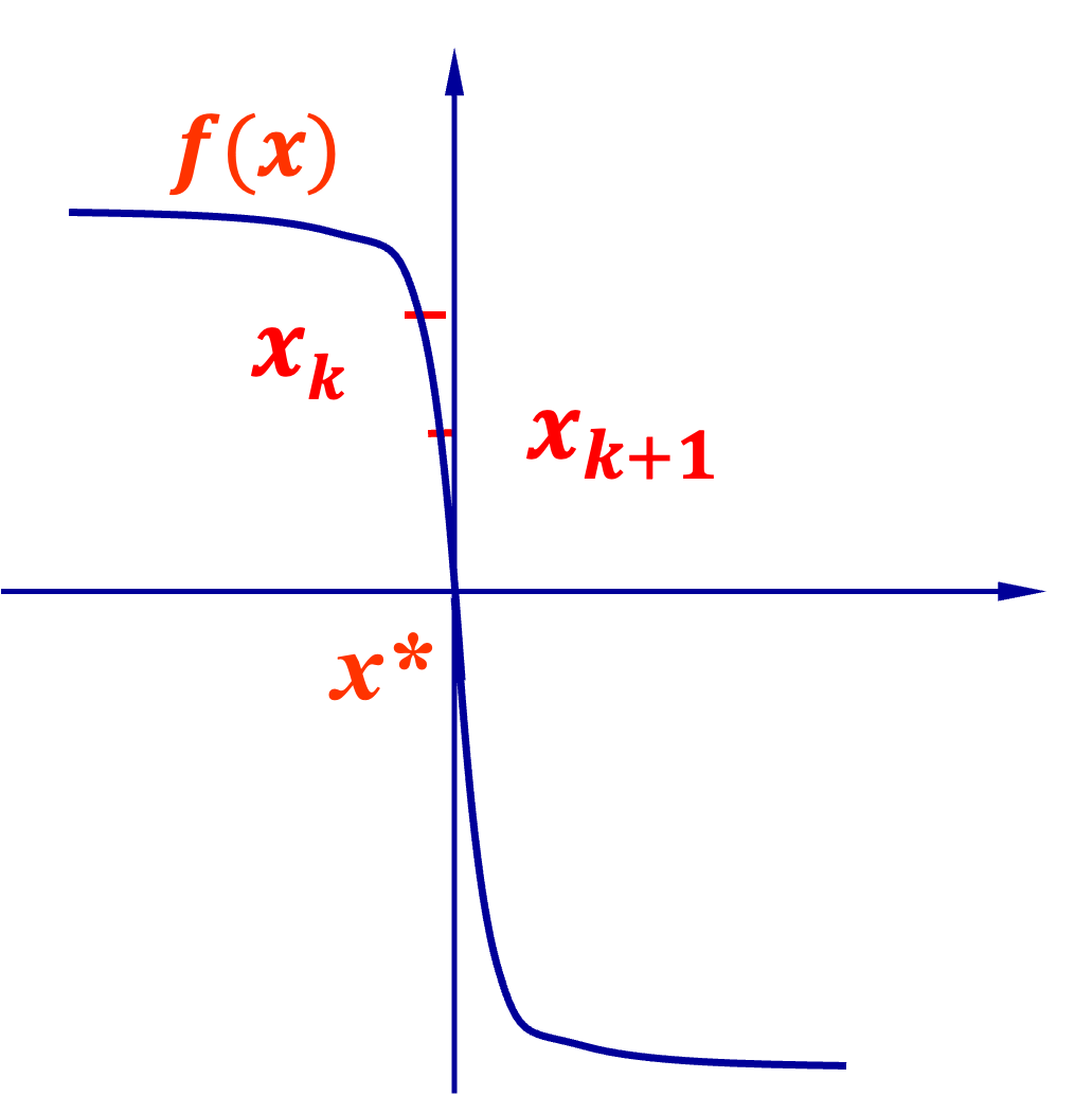 只用
只用