
1 偏微分方程介绍
任何一种随空间变化或随时空变化的物理现象(具有两个或以上自变量)都需要用偏微分方程描述。
偏微分方程的解法分为:
解析法:就是传统的理论推导演绎的方法。这种方法从物理问题所满足的偏微分方程出发,通过合理的简化,采用近似方法,降低求解难度,最终得出解析表达式,或者用
常用的
分离变量法 :通过分离变量法减少偏微分方程中的变量,将一个偏微分方程分解成若干个常微分方程。积分变换法 :利用积分法,将偏微分方程变换为可分离的偏微分方程,方便求解。一般为傅里叶变换分析。变量替换法 :通过适当的变量替换,可以简化偏微 分方程的求解。
\[ \partial_t V + \frac{1}{2}\sigma^2S^2\partial_S^2 V + rS\partial_S V -rV = 0 \] 通过如下变换: \[ \begin{matrix*}[l] V(S, t) = Kv(x\tau); \\ x = \ln(S/K); \\ \tau = \frac{1}{2}\sigma^2(T - t); \\ v(x, \tau) = \exp(-\alpha x - \beta \tau) u(x, \tau) \end{matrix*} \] 可以简化为热力学方程(扩散方程): \[ \partial_\tau u = \partial_x^2 u \]
1.1 Classification of PDE
大部分物理上重要的偏微分方程都是二阶的,它们的常见形式为: \[ AU_{xx} + 2BU_{xy} + CU_{yy} + DU_x + EU_y + FU = 0 \] 其中\(A,B,C\)等为参数并且取决于\(x,y\)。
如果在\(xy\)平面上有\(A^2 + B^2 + C^2 > 0\),且该偏微分方程在该平 平面上为二阶偏微分方程。
则该二阶偏微分方程可分类为:抛物型方程,双曲型方程和椭圆型方程,其分类方式为: \[\Delta \equiv B^2 - 4AC\]
- 若 \(\Delta < 0\),则为
椭圆型 方程; - 若 \(\Delta = 0\),则为
抛物型 方程; - 若 \(\Delta > 0\),则为
双曲型 方程
\[ \frac{dy}{dx} = \frac{B \pm \sqrt{B^2 - 4AC}}{2A} \tag{1}\]
| \[ B^2 - 4AC \] | characteristic line | kind |
|---|---|---|
| \[ <0 \] | complex | elliptical |
| \[ =0 \] | real, double | parabolic |
| \[ > 0 \] | real, single | hyperbolic |
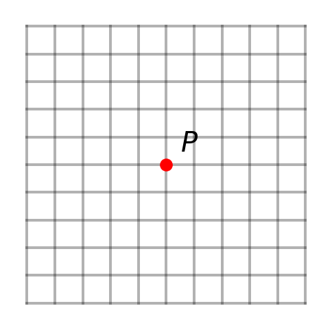
Poission eqn
Time-independent Schrodinger
\[ f_{xx} + f_{yy} = 0 \] \[ \frac{dy}{dx} = \pm i \]
Show the code
Relaxation methodDiffusion eqn
Time-dependent Schrodinger
\[ f_t - \alpha f_{xx} = 0 \]
\[ \frac{dy(x)}{dx(t)} = \infty \]
Show the code
plt.figure(figsize = (3, 3))
x = np.array([0, 1])
for i in range(6):
    y = np.array([1, 1]) * i * 0.1
    plt.plot(x, y, 'k-', alpha = 0.3)
for i in range(11):
    y = np.array([1, 1]) * i * 0.1
    x = np.array([0.5, 1])
    plt.plot(y, x, 'k-', alpha = 0.3)
plt.plot([0.5], [0.5], 'ro', lw = 8)
plt.text(0.55, 0.55, r'$P$', fontsize = 15)
plt.axis('off')
plt.show()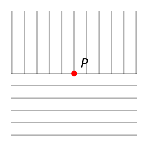
Forwardwave equation
EM wave
\[ f_{tt} - c^2f_{xx} = 0 \]
\[ \frac{dy(x)}{dx(t)} = \pm c \]
Show the code
plt.figure(figsize = (3, 3))
x = np.array([0, 1])
for i in range(6):
    y = np.array([1, 1]) * i * 0.1
    plt.plot(x, y, 'k-', alpha = 0.3)
for i in range(11):
    y = np.array([1, 1]) * i * 0.1
    x = np.array([0.5, 1])
    plt.plot(y, x, 'k-', alpha = 0.3)
plt.plot([0.5], [0.5], 'ro', lw = 8)
plt.text(0.5, 0.6, r'$P$', fontsize = 15)

y1 = np.array([0, 0.5])
y2 = np.array([1, 0.5])
x = np.array([0, 0.5])
plt.fill_between(x, y1, y2, color = 'k')
x = np.array([0.5, 1])
y1 = np.array([0.5, 0])
y2 = np.array([0.5, 1])
plt.fill_between(x, y1, y2, color = 'k')
plt.axis('off')
plt.show()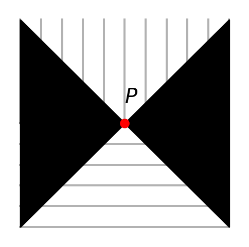
Forward因变量用它们在自变量的许多离散的格点上之值来描述, 通过适当的离散化,偏微分方程就化为一大组差分方程。
1.2 不同类型的偏微分方程举例
\[ \left\lbrace \begin{matrix*}[l] \nabla \cdot \vec{E} = \rho/\varepsilon \\ \nabla \cdot \vec{B} = 0 \\ \nabla \times \vec{E} = -\frac{1}{c}\frac{\partial \vec{B}}{\partial t} \\ \nabla \times \vec{B} = \frac{1}{c} \frac{\partial \vec{E}}{\partial t} + \mu_0 \vec{J} \end{matrix*} \right. \]
在静电场情况下,麦克斯韦方程组可写为 \[
\left\lbrace
\begin{matrix*}[l]
\nabla \cdot \vec{E} = \rho/\varepsilon \\
\nabla \times \vec{E} = 0
\end{matrix*}
\right.
\] 引入静电场的标量电势函数,并令 \(\vec{E} = -\nabla \phi\),可得静电场电势所满足的偏微分方程,即
求解泊松方程和拉普拉斯方程都需要给定场域的边界条件,构成电磁场的边值问题。
- 给定整个场域边界上的电势函数 \(\phi\) ,
第一类边值问题 - 给定边界上电势函数的法向微商\(\frac{\partial \phi_1}{\partial n}\big|_r\),
第二类边界问题 - 给定边界上电势函数与其法向微商的线性组合\(\phi + f \frac{\partial \phi_1}{\partial n}\big|_r\) 此为
第三类边界问题
- 抛物型偏微分方程 \(AU_{xx} + 2BU_{xy} + CU_{yy} + DU_x + EU_y +FU = 0\)
如果讨论电磁波在导电媒介中传播,其中位移电流的效应可以忽略时,电磁波方程可以写为
\[
\nabla^2 \vec{E} -\mu \gamma \frac{\partial \vec{E}}{\partial t} = 0
\] 方程归结为热传导方程,数学上属于
含时薛定谔方程: \[ -\frac{\hbar^2}{2m}\Psi_{xx}(x,t) + V(x)\Psi(x,t)=i\hbar\Psi_t(x,t) \]
- 双曲型偏微分方程
如果讨论电磁波在电介质中的传播,把电介质看作理想电介质 \((\gamma = 0)\),则电磁波方程可写为
\[ \nabla^2 \vec{E} - \mu \varepsilon \frac{\partial^2 \vec{E}}{\partial t^2} = 0 \] 或
\[ \nabla^2 \vec{E} - \mu \varepsilon \frac{\partial^2 \vec{E}}{\partial t^2} = \nabla \rho \] 电磁波方程归结为波动方程或弦振动方程,这两类方程在数学上属于双曲型偏微分方程。
1.3 偏微分方程的数值求解方法
有限差分法 :最早用于数值计算偏微分方程的计算方法,具有简明、直观的特点,但在快速计算机问世前,由于计算量大没有得到很好应用,现已成为一种有效方法。有限元素法(简称有限元法) :在有限差分法和变分法相结合的基础上发展出来的一种偏微分方程的计算方法。
我们将重点讲述如何用有限差分法数值求解偏微分方程。
因变量用它们在自变量的许多离散的格点上之值来描述,通过适当的离散化,偏微分方程就化为一大组差分方程。
2 差分法
用差分近似式替代导数,或用适当近似式替代含有导数的表达式,得到这些近似值满足的代数方程
节点 —— 正则内点,非正则内点
\(\longrightarrow\)
 \[h_i = \tau_i = h\]
 mesh slicing
例如:对单变量函数\(f(x)\),以步长\(h=\Delta x\)离散化,得到一系列节点\(x_i\)及相邻节点\(x_i-h, x_i+h\)。在节点的一阶向前、向后、中心差分分别为
\[ \begin{matrix*}[c] \frac{f(x_i + h) - f(x_i)}{h} \\ \frac{f(x_i) - f(x_i - h)}{h} \\ \frac{f(x_i + h) - f(x_i - h)}{2h} \end{matrix*} \] 可以类似地定义高阶差分差商。如二阶中心差商为 \[ \frac{f_{i + 1} - 2f_i + f_{i-1}}{h^2} \]
用何种差分格式,根据差分方程的
Example 1 常微分方程
\[ \left\lbrace \begin{matrix*}[l] y'' - x^2y= e^{-x}, ~~ x\in[0, 1] \\ y(0) = 0, ~~ y(1) = 1 \end{matrix*} \right. \] 取 \(h = (b - a)/n = 1/10, ~~ x_i = ih, ~~ i = 0,1,2,...,10\)

利用二阶中心差分公式 \(y_i'' = \frac{y_{i+1} - 2y_i + y_{i-1}}{h^2}\)
\[ \xrightarrow{\text{difference equation}} \left\lbrace \begin{matrix*}[l] y_{i+1} - (2+h^2x_i^2)y_i + y_{i-1} = h^2e^{-x_i} \\ y_0 = 0, ~~ y_{10} = 1, ~~ i = 1, 2, ..., 9 \end{matrix*} \right. \]

2.0.1 线性边值问题
\[ \left\lbrace \begin{matrix*}[l] y'' - x^2y = e^{-x}, ~ x \in [0, 1] \\ y(0) = 0, ~~ y(1) = 1 \end{matrix*} \right. \longrightarrow \left\lbrace \begin{matrix*}[l] y'' + p(x)y' + q(x)y = f(x) \\ y(a) = \alpha, ~~ y(b) = \beta \end{matrix*} \right. \] \[ \longrightarrow p = 0; ~~ q = -x^2; ~~ \alpha = 0; ~~ \beta = 1; ~~ f(x) = e^{-x} \]
\[ \begin{pmatrix} h^2q_1 - 2 & 1 & \\ 1 & h^2q_2 - 2 & 1 & \\ & \ddots & \ddots & \ddots \\ & & 1 & h^2q_8 - 2 & 1 \\ & & & 1 & h^2q_9 - 2 \end{pmatrix} \begin{pmatrix} y_1 \\ y_2 \\ \vdots \\ y_8 \\ y_9 \end{pmatrix} = \begin{pmatrix} h^2f_1-\alpha \\ h^2f_2 \\ \vdots \\ h^2f_8 \\ h^2f_9 - \beta \end{pmatrix} \]
%filename: chapter4_example_1_chafen.m
%用差分法求解线性边值问题,例题1
function chapter4_example_1_chafen
clear
clc
format long

XL=0.0;
XU=1;
N=100;           %取节点数,增加节点数,提高精度
h=(XU-XL)/N;
xx=XL:h:XL+N*h;

YL=0; YU=1;

A=zeros(N-1,N-1); %给系数矩阵赋值
A(1,1)=-2+h^2*(-h^2); A(1,2)=1; %将系数矩阵第一行和最后一行单独赋值
A(N-1,N-1)=-2+h^2*(-((N-1)*h)^2); A(N-1,N-2)=1;
for i=2:N-2       %对系数矩阵中中间行赋值
    A(i,i)=-2-h^2*(i*h)^2;
    A(i,i-1)=1;
    A(i,i+1)=1;
end

%给方程右边的列矩阵赋值
B=zeros(N-1,1);
B(1,1)=h^2*exp(-h)-YL;
B(N-1,1)=h^2*exp(-(N-1)*h)-YU;
for i=2:N-2
    B(i,1)=h^2*exp(-i*h);
end

yy=A\B;   %采用矩阵除法获得解得列矩阵

yy_cf(1)=YL;
yy_cf(N+1)=YU;
for i=2:N
   yy_cf(i)=yy(i-1,1);
end
yy_cf;

hold on
plot(xx,yy_cf,'b')%数值结果
title('差分法结果')
%filename: chapter4_example_1_shooting_method.m
%用打靶法求解常微分方程的边值问题,其中用到了弦割法和四阶R-K算法
function shooting_method_RK_secant
clear
clc
%close all
format long

DL=5*10^-19;  %误差判断标准,用于弦割法
XL=0.0;       %左边界点
XU=1.0;       %右边界点
h=0.01;
N=(XU-XL)/h;
xx=XL:h:XL+N*h;
%D = 1;               %初始化误差
YL= 0.0;              %左边界点函数值
YU= 1.0;              %右边界点函数值
S0= 85;              %XL处斜率的猜测值,弦割法第一个启动点
S1= 25;              %第二个斜率猜测值,作为弦割法的第二个启动点

%-----------四阶R-K算法,将求解放在循环外部-------------------
%---------第一个试探解,求右边界的函数值及误差函数-------------------
f=@(xx,yy)[yy(2);xx^2*yy(1)+exp(-xx)]; % 定义 f1,
z10 = [YL;S0];
z1 = myrungekutta(f, xx, z10);
y_rk1 = z1(1,:)';   %用四阶RK算法求得的y值
z_rk1 = z1(2,:)';
F0=y_rk1(end)-YU; %用四阶RK算法得到的XU点的函数值与边界条件的差值
%----------第二个试探解,求右边界的函数值及误差函数--------------------
z20 = [YL;S1];
z2 = myrungekutta(f, xx, z20);
y_rk2 = z2(1,:)';   %用四阶RK算法求得的y值
z_rk2 = z2(2,:)';
F1=y_rk2(end)-YU; %用四阶RK算法得到的XU点的函数值与边界条件的差值
if (abs(F1)>abs(F0))
    y_rk=y_rk1;
else
    y_rk=y_rk2;
end
nn=0; %迭代次数
%abs(y_rk(end)-YU)
while(abs(y_rk(end)-YU)>DL)
    nn=nn+1;
    S2=S1-F1*(S1-S0)/(F1-F0); %弦割法求根
    S0=S1;
    S1=S2;
    F0=F1;
    y_rk1=y_rk;
%----------第三或更高次的试探解,求右边界的函数值及误差函数--------------------
    z20 = [YL;S1];
    z2 = myrungekutta(f, xx, z20);
    y_rk2 = z2(1,:)';   %用四阶RK算法求得的y值
    z_rk2 = z2(2,:)';
    F1=y_rk2(end)-YU %用四阶RK算法得到的XU点的函数值与边界条件的差值
    if (abs(F1)>abs(F0))
        y_rk=y_rk1;
    else
        y_rk=y_rk2;
    end
    %abs(y_rk(end)-YU)
end
hold on
plot(xx,y_rk,'r')

function z = myrungekutta(f, xx, z0)
n = length(xx);
h = xx(2)-xx(1);
z(:,1)=z0;
for i = 1:n-1
    k1 = f(xx(i), z(:,i));
    k2=f(xx(i)+0.5*h, z(:,i) + h*k1/2);
    k3=f(xx(i)+0.5*h, z(:,i) + h*k2/2);
    k4=f(xx(i)+h, z(:,i) + h*k3);
    z(:,i+1)=z(:,i) + (k1 + 2*k2 + 2*k3 + k4)*h/6;
end
2.1 椭圆型偏微分方程
椭圆型方程最简单的形式就是Laplace方程 \(\Delta u = u_{xx} + u_{yy} = 0\) 它是如下的Possion方程的特殊情况 \[ \Delta u = u_{xx} + u_{yy} = S(x, y) \] 例如:我们将考虑二维空间 \((x, y)\) 内的场量\(\phi\)的椭圆型边值问题,方程为 \[ -[\partial_x^2 + \partial_y^2]\phi = S(x, y) \]
- Dirichlet问题 \(\phi|_G = g(p)\)
第一类边值问题 - Neumann问题 \(\frac{\partial \phi}{\partial n}\bigg|_G = g(p)\)
第二类边值问题 - 混合问题 \(\phi|_G + g_1(p) \frac{\partial \phi}{\partial n}\bigg|_G = g_2(p)\)
第三类边值问题

取 Dirichlet 型边界条件(第一类边值问题),为方便起见边界线取为单位正方形,边值问题就是要用方程求出单位正方形内每处的\(\phi\)。
首先定义一个网格,覆盖\((x, y)\)平面内的单位正方形。为方便起见,我们取格子间隔 \(h\) (步长)是均匀的,并且在两个方向上相等,使得单位正方形被 \((N+1) \times (N+1)\) 个格点覆盖。这些格点用指标 \((i, j)\) 编号,其中 \(i, j = 0,1,2,3, ..., N\)。
Show the code
plt.figure(figsize = (5, 5))
x = np.array([0, 1])
for i in range(11):
    y = np.array([1, 1]) * i * 0.1
    plt.plot(x, y, 'k-', alpha = 0.3)
    plt.plot(y, x, 'k-', alpha = 0.3)
plt.text(-0.1, -0.05, r'$x = 0$', fontsize = 15)
plt.text(0.9, -0.05, r'$x = 1$', fontsize = 15)
plt.text(-0.3, -0.05, r'$y = 0$', fontsize = 15)
plt.text(-0.15, 0.97, r'$y = 1$', fontsize = 15)
plt.axis('off')
plt.show()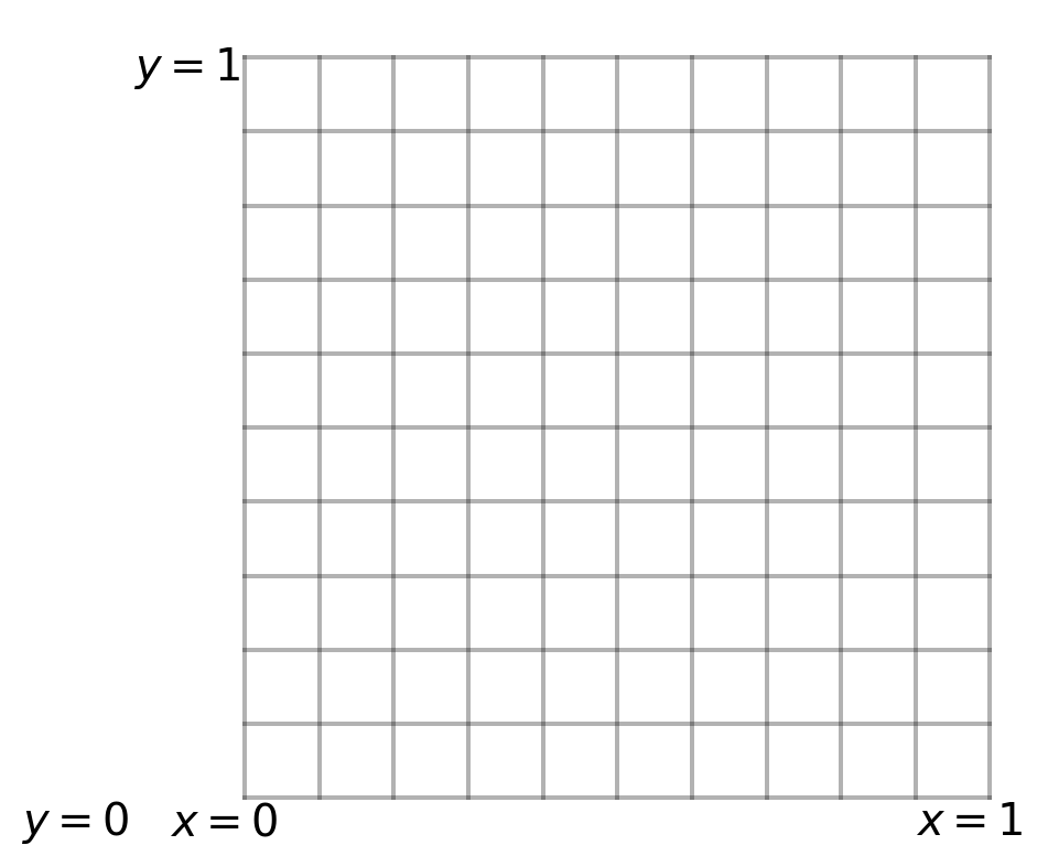
2.1.1 将场域离散化
把偏导数用节点上的函数值表示出来,分别以\(f_0, f_1, f_2, f_3, f_4\), 代表在\(0, 1-4\) 的函数值

由1,3点值给出 \(\left( \frac{\partial \phi}{\partial x} \right)_0 \approx \frac{\phi_1 - \phi_0}{h_1} ~~~~~ \left( \frac{\partial \phi}{\partial x} \right)_0 \approx \frac{\phi_0 - \phi_3}{h_3}\)
显然,这种单侧差商误差较大,引入\(a, b\),由\(f_1\)和\(f_3\) 的泰勒展开式,可构造出下面的关系式(考虑到\(h_1\)与\(h_3\)可能不同)
\[ \alpha(\phi_1 - \phi_0) + \beta(\phi_3 - \phi_0) = \left( \frac{\partial \phi}{\partial x} \right)_0 (\alpha h_1 - \beta h_3) + \frac{1}{2}\left( \frac{\partial^2 \phi}{\partial x^2} \right)_0(\alpha h_1^2 + \beta h_3^2) + ... \]
令第二项系数为零,得 \[ \alpha = -\frac{h_3^2}{h_1^2}\beta \longrightarrow \left(\frac{\partial \phi}{\partial x}\right) \approx \frac{h_3^2(\phi_1 - \phi_0) - h_1^2(\phi_3 - \phi_0)}{h_1h_3(h_3 + h_1)} = \frac{\phi_1 - \phi_3}{2h} \]
继续推导二阶偏导数的差分表达式,在泰勒展开式里,令第一项系数为零,则有 \(\alpha = - \frac{h_3}{h_1}\beta\)
忽略三阶以上高次项,有
\[ \left(\frac{\partial^2 \phi}{\partial x^2}\right)_0 \approx 2\frac{h_1(\phi_1 - \phi_0) + h_3(\phi_3 - \phi_0)}{h_1h_3(h_3 + h_1)} = \frac{\phi_1 - 2\phi_0 + \phi_3}{h^2} \]
用完全相同的方法可以确定 \(y\) 方向
\[
\left(\frac{\partial^2 \phi}{\partial y^2}\right)_0 \approx 2\frac{h_2(\phi_2 - \phi_0) + h_4(\phi_4 - \phi_0)}{h_2h_4(h_2 + h_4)} = \frac{\phi_2 - 2\phi_0 + \phi_4}{h^2}
\] 误差为
\[ \longrightarrow -\Delta\phi = - \left[ \frac{\phi_1 -2\phi_0 + \phi_3}{h^2} + \frac{\phi_2 -2\phi_0 + \phi_4}{h^2} \right] = S_0 \]
\[ - \left[ \frac{\phi_1 -2\phi_0 + \phi_3}{h^2} + \frac{\phi_2 -2\phi_0 + \phi_4}{h^2} \right] = S_0 \]
\[ \Longrightarrow - \left[ \frac{\phi_{i+1, j} -2\phi_{i,j} + \phi_{i-1,j}}{h^2} + \frac{\phi_{i,j+1} -2\phi_{i,j} + \phi_{i,j-1}}{h^2} \right] = S_{i,j} \]
\[ - \left[ \frac{\phi_{i+1, j} -2\phi_{i,j} + \phi_{i-1,j}}{h^2} + \frac{\phi_{i,j+1} -2\phi_{i,j} + \phi_{i,j-1}}{h^2} \right] = S_{i,j} \]
\[ -[(\delta_i^2\phi)_{ij} + (\delta^2_j\phi)_{ij}] = h^2S_{ij} ~~~~ \Longleftrightarrow ~~~~\left\lbrace \begin{matrix*}[l] (\delta_i^2\phi)_{ij} \equiv \phi_{i+1, j} + \phi_{i-1, j} -2\phi_{ij} \\ (\delta_j^2\phi)_{ij} \equiv \phi_{i, j+1} + \phi_{i, j-1} -2\phi_{ij} \end{matrix*} \right. \]
对于二维Laplace方程 \(\phi_{xx} + \phi_{yy} = 0\)
\[ -[\phi_{i+1, j} + \phi_{i-1, j} + \phi_{i, j+1} + \phi_{i, j-1} - \phi_{i, j}] = 0 \] 显式迭代: \[ \phi_{ij} = \frac{1}{4}[\phi_{i+1, j} + \phi_{i-1, j} + \phi_{i, j+1} + \phi_{i, j-1}] \] see (Figure 1)
对微分方程的离散近似等价于关于区域的内点上的未知 \(f\) 值的一个线性方程组。用矩阵记号,它可以写为 \[ A\phi = B \] 其中 \(A\) 是出现在线性方程组中的矩阵, \(\phi\) 表示内点上的 \(f\) 值,非齐次项 \(B\) 包含内点上的 \(S\) 以及边界上的 \(f\) 值。
\(f\) 可以通过矩阵求逆来获得 \(\phi = A^{-1}B\)
\[ 2\phi_i - \phi_{i+1} - \phi_{i - 1} = h^2S_i ~~\Longrightarrow ~~ A\phi = B \]
与线性常微分方程差分格式的比较
\[ A_{ij} = \left\lbrace \begin{matrix*}[l] 2 ~~\text{for}~~ i = j; ~~~~ B_i = h^2S_i ~~\text{for}~~i\in[2,N-2] \\ -1 ~~\text{for}~~ i = j\pm 1; ~~~~ B_1 = h^2S_1 + \phi_0 \\ 0 ~~\text{otherwise}; ~~~~~~ B_{N-1} = h^2S_{N-1} + \phi_N \end{matrix*} \right. \]
\[ \phi = \begin{pmatrix} \phi_1 \\ \phi_2 \\ \vdots \\ \phi_{N-2} \\ \phi_{N-1} \end{pmatrix}, A = \begin{pmatrix} 2 & -1 & 0 & 0 & \dots & 0 & 0 & 0 \\ -1 & 2 & -1 & 0 & \dots & 0 & 0 & 0 \\ 0 & -1 & 2 & -1 & \dots & 0 & 0 & 0 \\ & & \dots & & \ddots & & \dots & & \\ 0 & 0 & 0 & 0 & \dots & -1 & 2 & -1 \\ 0 & 0 & 0 & 0 & \dots & 0 & -1 & 2 \end{pmatrix}, B = \begin{pmatrix} h^2S_1 + \phi_0 \\ h^2S_2 \\ \vdots \\ h^2S_{N-2} \\ h^2S_{N-1}+\phi_{N-1} \end{pmatrix}, \]
当点数不太多时,我们可以利用矩阵求逆的方法来求解
2.1.1.1 二维问题的差分格式
\[ \left\lbrace \begin{matrix*} u_{xx} + u_{yy} = 0, ~~ (x, y) \in D \\ u(x, y) = \log[(1 + x)^2 + y^2], ~~ (x, y) \in \partial D \end{matrix*} \right. \] \(D = \{ (x, y)|0 \leq x, y \leq 1 \}\)
\[ -[\phi_{i+1, j} + \phi_{i-1, j} + \phi_{i, j+1} + \phi_{i, j-1} -4\phi_{i,j}] = 0 \]
\[ -\left[ \frac{\partial^2}{\partial x^2} + \frac{\partial^2}{\partial y^2} \right] \phi = 0 \]
取特殊的网格 \(h=1/3\), 如右图,求差分方程的矩阵形式

差分方程的矩阵形式为
\[ \begin{pmatrix} 4 & -1 & -1 & 0 \\ -1 & 4 & 0 & -1 \\ -1 & 0 & 4 & -1 \\ 0 & -1 & -1 & 4 \end{pmatrix} \begin{pmatrix} u_1 \\ u_2 \\ u_3 \\ u_4 \end{pmatrix} = \begin{pmatrix} \alpha_1 + \alpha_8 \\ \alpha_2 + \alpha_3 \\ \alpha_6 + \alpha_7 \\ \alpha_4 + \alpha_5 \end{pmatrix} \] 其中 \(\alpha(x, y) = \log[(1+x)^2 + y^2]\), \(\alpha_1\)为\(B_1\)点处的函数值,其他类推
解得:
$ u_1 = 0.634804,~~ u_2 = 1.059993,~~ u_3 = 0.798500,~~u_4 = 1.169821$
2.2 迭代法
当格点取得非常密时,选择矩阵求逆的方法来求解是非常不明智的,所以寻求一种适用于更高维数的、效率更高的算法是非常重要的。由于对Laplace 算符的离散近似只包含相邻的点,\(A\)为稀疏矩阵,可以采用高效的迭代法求解。
以一维问题为例,其差分方程为 \(2\phi_i - \phi_{i+1} - \phi_{i-1} = h^2S_i\)
这里采用迭代法来求解。首先将上式改写为“解出” \(\phi_i\) 的形式 \(\phi_i = \frac{1}{2}[\phi_{i+1} + \phi_{i-1} + h^2S_i]\)
2.2.1 Jacobi迭代法
Jacobi迭代法的思想:先猜测一个初始解 \(\phi^0\),然后根据下面的递推关系生成一系列的解,直到收敛为止。
\[ \phi_i^{n+1} = \frac{1}{2}[\phi_{i+1}^n + \phi_{i-1}^n + h^2S_i^b] \tag{2}\]
(\(n\)为迭代次数)可以证明,不论初始值 \(\phi^0\) 如何选取,当\(n \rightarrow \infty\)时, \(\phi^{n+1}\) 必然收敛于差分问题的解。
上述方法中,计算第\(n+1\)次的第\(i\)点的值时所用到的相邻点的值,是前一次(第\(n\)次)的计算结果。因此必须等到第\(n\)次所有点的值计算完毕,才能进行下一次运算。这种算法又称为
从下面的例题2与3将可以看出,
Example 2 用显式差分公式求解平面温度场
设正方形场域的一边温度为\(10~{}^\circ \text{C}\),其余各边的温度均为\(0~{}^\circ \text{C}\),求稳定的温度场。
定解问题是 \[ \left\lbrace \begin{matrix*}[l] u_{xx} + u_{yy} = 0; ~~ x \in [0, 100], ~~ y\in [0, 100]; \\ u(0, y) = 0, ~~ u(100, y) = 10; \\ u(x, 0) = 0,~~ u(x, 100) = 0 \end{matrix*} \right. \]
\[ u_{ij} = \frac{1}{4}[u_{i+1,j} + u_{i-1, j} + u_{i,j+1}+u_{i,j-1}] \tag{3}\] 三条边的值为\(0\),一条为\(10\),平均的粗略地取\(10/4=2.5\)作为内节点的初始值(计算的启动值),取迭代误差值小于\(0.01\)。
注意矩阵最大值的求法:A中的最大元素为max(max(A))
%filename: chapter4_example_2_temperature.m
clear
close all
clc
%example-2,求解温度场

u=zeros(101,101);
u(101,:)=10; %边界条件,其他三个边界条件包含在u的初始定义里
uold=u;
u(2:100,2:100)=u(2:100,2:100)+12.5;
nn=0;
while max(max(abs(u-uold)))>=0.00000001
      uold=u;
      u(2:100,2:100)=0.25*(u(3:101,2:100)+u(1:99,2:100)+u(2:100,3:101)+u(2:100,1:99));
      nn=nn+1;
end
max(max(abs(u-uold)))
nn
figure,surf(u)
figure,contour(u)
%filename: chapter4_example_2_temperature_1.m
clear
close all
clc
%example-2,求解温度场;
%利用此程序验证:不同初始猜测对收敛速度有影响,但对结果基本没有影响
N=100;
u=zeros(N+1,N+1);
u(N+1,:)=10; %边界条件
u1=u;
uold=u;
uold_1=u1;
u(2:N,2:N)=u(2:N,2:N)+2.5; %不同初始猜测对收敛速度有影响,但对结果基本没有影响
u1(2:N,2:N)=u1(2:N,2:N)+17.1;
nn=0;
tic
while max(max(abs(u-uold)))>=0.0000001
uold=u;
u(2:N,2:N)=0.25*(u(3:N+1,2:N)+u(1:N-1,2:N)+u(2:N,3:N+1)+u(2:N,1:N-1));
nn=nn+1;
end
toc
nn
mm=0;
tic
while max(max(abs(u1-uold_1)))>=0.0000001
uold_1=u1;
u1(2:N,2:N)=0.25*(u1(3:N+1,2:N)+u1(1:N-1,2:N)+u1(2:N,3:N+1)+u1(2:N,1:N-1));
mm=mm+1;
end
toc
mm
figure,surf(u);
figure,[c,h]=contour(u,20);
set(h,'ShowText','on','TextStep',get(h,'LevelStep')*2);
colormap cool
title('温度场的平面等高图')
figure;surf(u-u1)Show the code
import numpy as np
from mpl_toolkits.mplot3d import Axes3D
import matplotlib.pyplot as plt

u = np.zeros((101, 101))
u[-1, :] = 10.0 #边界条件,其他三个边界条件包含在u的初始定义里
uold = u.copy()
u[1:-1, 1:-1] = u[1:-1, 1:-1] + 12.5
nn = 0
while np.max(np.max(np.abs(u-uold)))>=0.00000001:
    uold=u.copy()
    u[1:-1,1:-1]=0.25*(u[2:,1:-1]+u[0:-2,1:-1]+u[1:-1,2:]+u[1:-1,0:-2])
    nn=nn+1

fig = plt.figure(figsize = (10, 4))
ax = fig.add_subplot(121, projection='3d')
x = y = np.linspace(0, 1, 101)
X, Y = np.meshgrid(x, y)

ax.plot_surface(X, Y, u, cmap = 'jet')

ax.set_xlabel('X Label')
ax.set_ylabel('Y Label')
ax.set_zlabel('Z Label')

plt.subplot(122)
plt.imshow(u, cmap = 'jet')
plt.colorbar()
plt.show()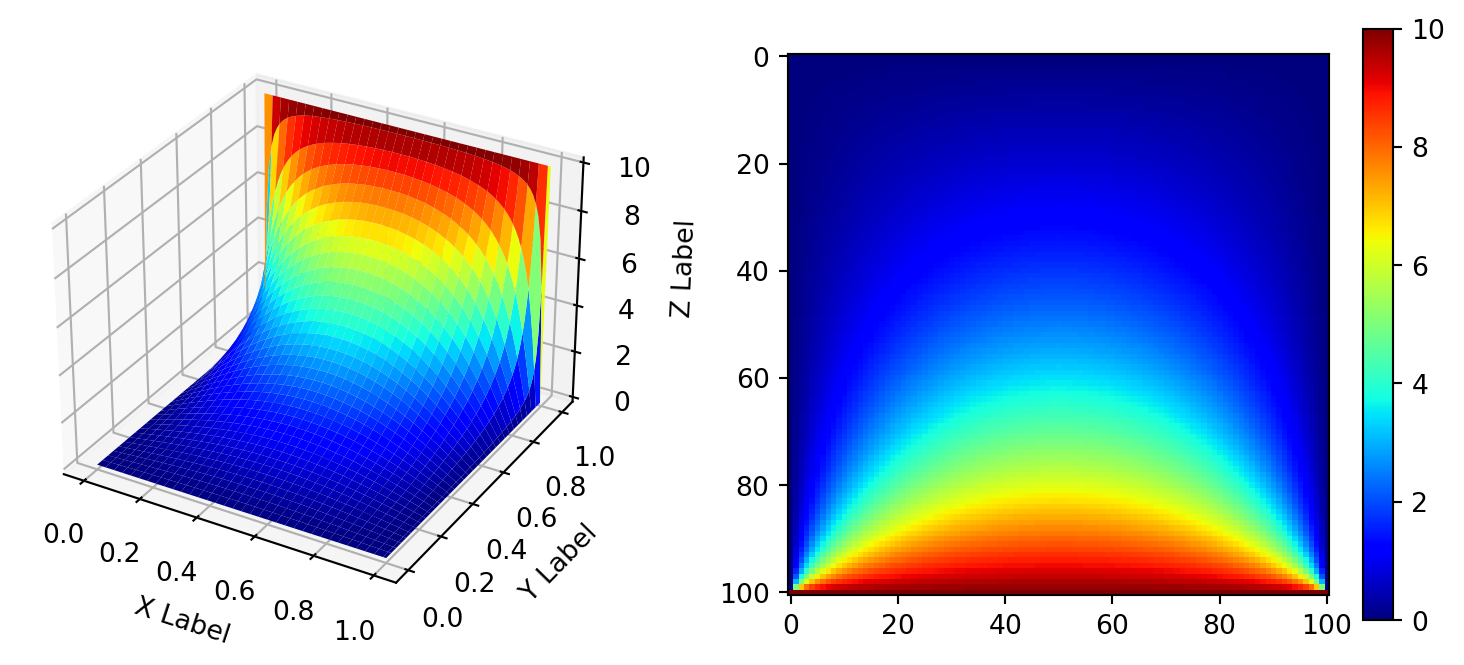
Example 3 求平面(正方形场域)温度场
定解问题是 \[ \left\lbrace \begin{matrix*}[l] u_{xx} + u_{yy} = 0; ~~ x \in [0, a], ~~ y\in [0, b]; \\ u(0, y) = 0, ~~ u(a, y) = \mu \sin \frac{3\pi y}{b}; \\ u(x, 0) = 0,~~ u(x, b) = \mu \sin\frac{3\pi x}{a} \cos\frac{\pi x}{a} \end{matrix*} \right. \tag{4}\] with \(\mu = 1, ~~a = 3, ~~b = 2\)
Refer (Equation 3)
\[\begin{eqnarray} u(x, y) &=& \frac{\mu}{2} \left[ \frac{1}{\sinh\frac{2\pi b}{a}} \sinh\frac{2\pi y}{a} \sin\frac{2\pi x}{a} + \frac{1}{\sinh\frac{4\pi b}{a}} \sinh\frac{4\pi y}{a} \sin\frac{4\pi x}{a} \right] + \mu \frac{1}{\sinh\frac{3\pi a}{b}} \sinh\frac{3\pi x}{b} \sin\frac{3\pi y}{b} \\ &=& \frac{1}{2} \left[ \frac{1}{\sinh\frac{4\pi}{3}} \sinh\frac{2\pi y}{3} \sin\frac{2\pi x}{3} + \frac{1}{\sinh\frac{8\pi}{3}} \sinh\frac{4\pi y}{3} \sin\frac{4\pi x}{3} \right] + \frac{1}{\sinh\frac{9\pi}{2}} \sinh\frac{3\pi x}{2} \sin\frac{3\pi y}{2} \end{eqnarray}\]Code:
%filename: chapter4_example_3_temperature.m
clear all
close all
clc
%example-3,求解温度场;
a=3;b=2;h=0.05;
x=0:h:a;
y=0:h:b;
[X,Y]=meshgrid(x,y);
Z=0.5*(1/sinh(2*pi*b/a)*sinh(2*pi*Y/a).*sin(2*pi*X/a)+...
    1/sinh(4*pi*b/a)*sinh(4*pi*Y/a).*sin(4*pi*X/a))+...
    1/sinh(3*pi*a/b)*sinh(3*pi*X/b).*sin(3*pi*Y/b);
figure;surf(X,Y,Z);
title('解析法得到的温度场的三维图')
figure;contour(X,Y,Z,20); %控制等高线的条数
title('解析法得到的温度场的等高图')

figure; meshc(X,Y,Z);
colormap hsv
title('解析法得到的温度场的三维图与等高图')
%============数值解-有限差分法===========================
XL=0;XR=a;
YL=0;YR=b;
N=(XR-XL)/h;
M=(YR-YL)/h;
u=zeros(N+1,M+1);
u(N+1,1:M+1)=sin(3*pi/b*(0:M)*h); %边界条件
u(1:N+1,M+1)=sin(3*pi/a*(0:N)*h).*cos(pi/a*(0:N)*h);
uold=u;
u(2:N,2:M)=u(2:N,2:M)+2; %启动值
nn=0;
while max(max(abs(u-uold)))>=10^-10
        %由于u矩阵为二维,故矩阵最大值的求解利用了两重max算法
        uold=u;
        u(2:N,2:M)=0.25*(u(3:N+1,2:M)+u(1:N-1,2:M)+u(2:N,3:M+1)+u(2:N,1:M-1));
        nn=nn+1;
end

%figure; surf(X,Y,u')
%figure; contour(X,Y,u',20)
nn
u_error=u'-Z;
figure; meshc(X,Y,u');
colormap hsv
title('差分法得到的温度场的三维图与等高图')
figure; surf(X,Y,u_error)
title('差分法与解析法的误差')
Show the code
u = np.zeros((301, 201))
x = np.linspace(0, 3, 301)
y = np.linspace(0, 2, 201)
u[-1, :] = np.sin(3.0 * np.pi * y / 2.0)
u[:, -1] = np.sin(3.0 * np.pi * x / 3.0) * np.cos(np.pi * x / 3.0)
uold = u.copy()
u[1:-1, 1:-1] = u[1:-1, 1:-1] + 12.5
nn = 0
while np.max(np.max(np.abs(u-uold)))>=0.00000001:
    uold=u.copy()
    u[1:-1,1:-1]=0.25*(u[2:,1:-1]+u[0:-2,1:-1]+u[1:-1,2:]+u[1:-1,0:-2])
    nn=nn+1

fig = plt.figure(figsize = (10, 4))
ax = fig.add_subplot(121, projection='3d')
X, Y = np.meshgrid(y, x)

ax.plot_surface(X, Y, u, cmap = 'jet')

ax.set_xlabel('X Label')
ax.set_ylabel('Y Label')
ax.set_zlabel('Z Label')

plt.subplot(122)
plt.imshow(u, cmap = 'jet')
plt.colorbar()
plt.show()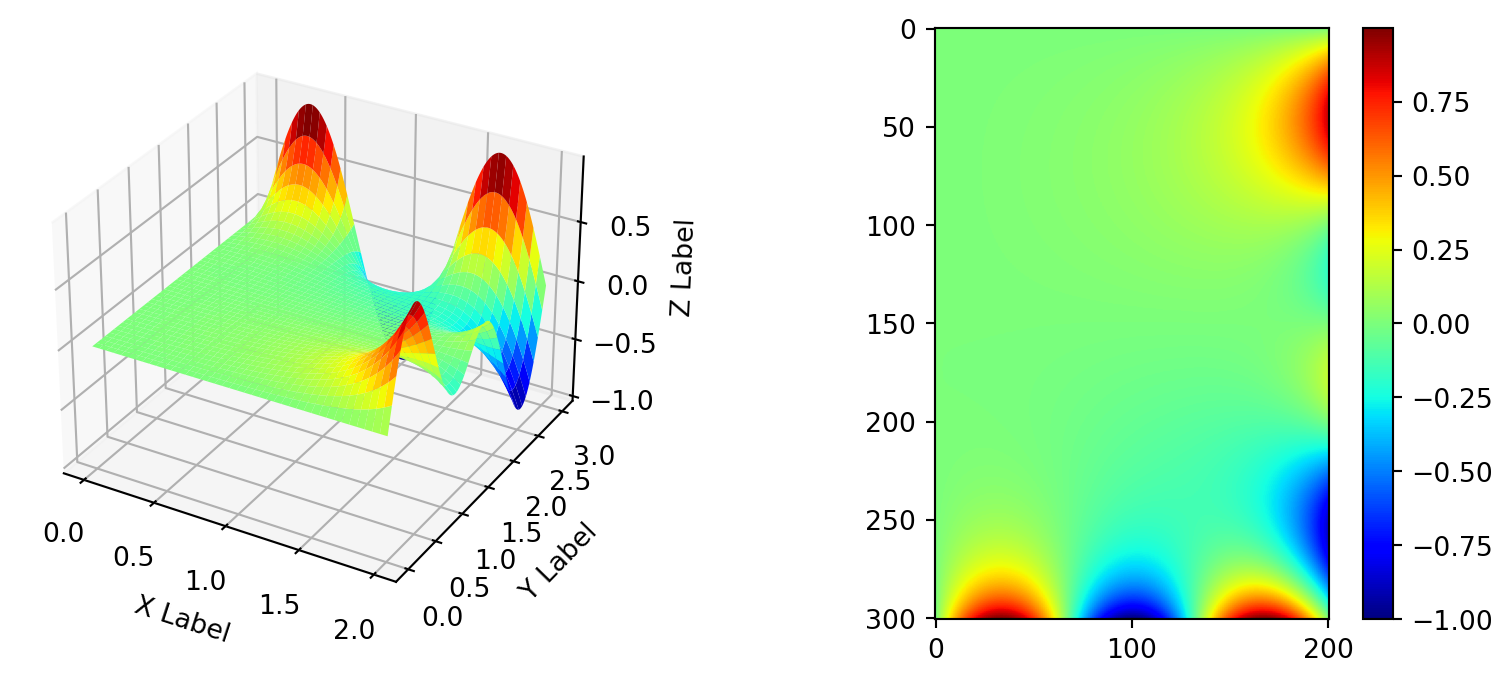
2.2.2 Gauss-Seidel 迭代法
在这种迭代法中,如果进行某个内点的第\(n+1\)次迭代式,某些相邻点的第\(n+1\)次近似值已经计算出,那么在计算中就用这个新值代替旧值,此时迭代公式为
\[
\phi_i^{n+1} = \sum_{j<i}a_{ij}\phi_j^{n+1} + \sum_{j>i}a_{ij}\phi_j^n + h^2S_i^n
\] 应用到一维问题的Jacobi迭代中为 \[
\phi_i^{n+1} = \frac{1}{2}[\phi_{i+1}^n + \phi_{i-1}^{n+1} + h^2S_i^n]
\tag{5}\] Gauss-Seidel迭代法可以提高迭代的效率。如果我们将每次计算的新值替换成新值与旧值的某种“组合”,将获得下面更高效率的基于Gauss-Seidel迭代法的松弛法的公式。 \[
\phi_i^{n+1} = (1-\omega)\phi_i^n + \frac{1}{2}\omega[\phi_{i+1}^n + \phi_{i-1}^{n+1} + h^2S_i^n]
\tag{6}\] Gauss-Seidel 迭代法又可以称为
对于
- \(\omega > 1\) 对应于“超松弛”
- \(\omega < 1\) 则意味“低松弛”

- 从一个
良好的猜测 解出发会减少所需的迭代次数 - 使用
松驰因子的最优值 (可以用解析方法来估计,也可以用经验方法来决定)。一般的分析表明,松弛参数的最佳选择依赖于格子大小和问题的几何条件。它通常大于1,接近2 。最佳值可以由经验方式决定,这只要在选择一个供多次迭代使用的参数值之前考察解在前几次迭代中的收敛情况就可以了。 - 在几次迭代中,把松驰过程集中在网格的一子区域(已知试验解在这个区域中特别不好)中进行, 这样就不会在解的已松驰部分浪费力量。
- 可以先在比较粗的网格上进行计算,它经过 少量的计算工作之后就会松驰,然后再把求得的解内插到一个更精细的网格上,将其用作进一步迭代的起始猜测。
2.3 二维椭圆型方程的松弛法
将松弛法推广到高维是非常直接的。以二维为例,差分方程为 \[ -\left[ \frac{\phi_{i+1, j} + \phi_{i-1, j} - 2\phi_{ij}}{h^2} + \frac{\phi_{i, j+1} + \phi_{i, j-1} - 2\phi_{ij}}{h^2} \right] = S_{ij} \]
\[ \Longrightarrow \phi_{ij} = \frac{1}{4}\left[ \phi_{i-1,j} + \phi_{i+1,j} + \phi_{i, j+1} + \phi_{i, j-1} + h^2S_{ij} \right] \] \[ \xrightarrow{\text{Gauss-Seidel}} \phi_{ij}^{n+1} = \frac{1}{4}\left[ \phi_{i+1,j}^{n}+ \phi_{i-1,j}^{n+1} + \phi_{i, j+1}^{n} + \phi_{i, j-1}^{n+1} + h^2S_{ij}^n \right] \] 相应的松弛法格式为 \[ \phi_{ij} \longrightarrow \phi_{ij}^{n+1} = (1-\omega)\phi_{ij}^n + \frac{\omega}{4}\left[ \phi_{i+1,j}^{n}+ \phi_{i-1,j}^{n+1} + \phi_{i, j+1}^{n} + \phi_{i, j-1}^{n+1} + h^2S_{ij}^n \right] \]
Example 4 求平面(正方形场域)温度 Refer (Equation 4)
\[ u_{ij}^{n+1} = u_{ij}^n + \frac{\omega}{4}\left[ u_{i+1,j}^{n}+ u_{i-1,j}^{n+1} + u_{i, j+1}^{n} + u_{i, j-1}^{n+1} -4u_{ij}^n \right] \]
%filename: chapter4_example_4_temperature_Gauss_Seidel.m
%example-4,用松弛法(Gauss-Seidel迭代法)求解温度场
clear all
close all
clc

a=3;b=2;h=0.05;
%===========解析结果======================
x=0:h:a;
y=0:h:b;
[X,Y]=meshgrid(x,y);
Z=0.5*(1/sinh(2*pi*b/a)*sinh(2*pi*Y/a).*sin(2*pi*X/a)+...
    1/sinh(4*pi*b/a)*sinh(4*pi*Y/a).*sin(4*pi*X/a))+...
    1/sinh(3*pi*a/b)*sinh(3*pi*X/b).*sin(3*pi*Y/b);
figure(1),surf(X,Y,Z)
title('解析法得到的温度场的三维图')
%=================数值解==========================
XL=0;XR=a;
YL=0;YR=b;
N=(XR-XL)/h;
M=(YR-YL)/h;
u=zeros(N+1,M+1);
u(N+1,1:M+1)=sin(3*pi/b*(0:M)*h); %边界条件
u(1:N+1,M+1)=sin(3*pi/a*(0:N)*h).*cos(pi/a*(0:N)*h); %边界条件
u(2:N,2:M)=u(2:N,2:M)+2.0;                    %初始猜测值
%unew=u;
omega=0.9; %松弛因子,omega=1时为gauss-seidel迭代法
n=0; %迭代次数
err=1;
    while abs(err)>=10^-10
        n=n+1;
        err=0;
        for i=2:N
            for j=2:M
                %Gauss-Seidel迭代法
                relx=omega/4*(u(i,j+1)+u(i,j-1)+u(i+1,j)+u(i-1,j)-4*u(i,j));
                u(i,j)=u(i,j)+relx;
                if abs(relx)>err
                    err=abs(relx);
                end
                %err=abs(relx/omega);
            end
        end
    end

n
abs(err)
figure(2); surf(X,Y,u')
title('Gauss-Seidel迭代法得到的温度场的三维图')
u_error=u'-Z;
figure(3); surf(X,Y,u_error)
title('数值方法与解析方法的误差')
Example 5 利用松弛法求解下述偏微分方程 \[ \left\lbrace \begin{matrix*}[l] -\left( \partial_x^2 + \partial_y^2 \right) \phi = S(x, y), ~~ (0<x<1, 0<y<1) \\ \phi(0, y) = \sin y^2, ~~ \phi(1, y) = \sin(y^2 + 1) \\ \phi(x, 0) = \sin x^2, ~~ \phi(x, 1) = \sin(x^2 + 1) \end{matrix*} \right. \] 其中 \(S(x, y) = -4\cos(x^2 + y^2) + 4(x^2 + y^2)\sin(x^2 + y^2)\)
精确解为 \(\phi(x, y) = \sin(x^2 + y^2)\)
泊松方程的差分格式 \[ -[\phi_{i+1, j} + \phi_{i-1, j} + \phi_{i, j+1} + \phi_{i, j-1} - 4\phi_{ij}] = h^2S_{ij} \]
%filename: chapter4_example_5.m
close all
clc
%example-5 用松弛法(Gauss-Seidel迭代法)求偏微分方程;

a=1;b=1;h=0.01;
%===========解析结果======================
x=0:h:a;
y=0:h:b;
[X,Y]=meshgrid(x,y);
Z=sin(X.^2+Y.^2);
%=================解析结果的另一种赋值方法==========================
XL=0;XR=a;
YL=0;YR=b;
N=(XR-XL)/h;
M=(YR-YL)/h;
u_r=zeros(N+1,M+1);
for i=1:M+1
    u_r(1:N+1,i)=sin((0:N).^2*h^2+(i-1)^2*h^2);
end
%=================数值解==========================
u=zeros(N+1,M+1);
u(1,1:M+1)=sin((0:M).^2*h^2);%边界条件
u(N+1,1:M+1)=sin((0:M).^2*h^2+1);%边界条件
u(1:N+1,1)=sin((0:N).^2*h^2);%边界条件
u(1:N+1,M+1)=sin((0:N).^2*h^2+1); %边界条件
%给S赋值
S1=-4*cos(X.^2+Y.^2)+4*(X.^2+Y.^2)*sin(X.^2+Y.^2);
%给S赋值的另一种写法
for i=1:M+1
S(1:N+1,i)=-4*cos((0:N).^2*h^2+(i-1)^2*h^2)...
              +4*((0:N).^2*h^2+(i-1)^2*h^2).*sin((0:N).^2*h^2+(i-1)^2*h^2);
end

u(2:N,2:M)=u(2:N,2:M)+4.5;  %初始猜测值,改变初始值对结果没有影响
%uold=u;
omega=1.90; %松弛因子
n=0; %迭代次数
err=1;
    while abs(err)>=10^-10 %收敛判断标准
        n=n+1;
        err=0;
        for i=2:N
            for j=2:M
                relx=omega/4*(u(i,j+1)+u(i,j-1)+u(i+1,j)+u(i-1,j)+h^2*S(i,j)-4*u(i,j));
                u(i,j)=u(i,j)+relx;
                if abs(relx)>err
                    err=abs(relx);
                end
            end
        end
    end

error=u_r-u';   %与精确值间的误差
error1=Z-u';    %与精确值间的误差的另一种写法

n
err
max(max(error))
hold on
surf(X,Y,Z)
figure;surf(X,Y,error)

%figure; contourf(u)
%figure; contourf(u_r)
%colorbar
3 抛物型偏微分方程
在物理学中遇到的典型的抛物型偏微分方程有扩散方程 \[ \Phi_t = \nabla \cdot(\underbrace{D}_{\text{diffusion term}}\nabla \Phi)+\underbrace{S}_{\text{source term}} \tag{7}\] 含时薛定谔方程 \[ i\hbar\Phi_t = -\frac{\hbar^2}{2m}\nabla^2\Phi + V\Phi \tag{8}\]
与椭圆型方程的边值问题不同,抛物型方程一般都是初值问题,即,给出一个初始时刻的 \(\Phi\) 场,我们要求随后某时刻的 \(\Phi\) 场,其演化要服从一定的空间边界条件, 例如,在一些界面上规定了温度或热通量,或者在远距离处薛定谔方程的波函数变为
抛物型偏微分方程求解的是满足一定空间边界条件的初值问题,又称
- 先讨论最简单的一维扩散问题(Equation 7)
- 假定扩散系数 \(D\) 不随空间变化,不妨设其为\(1\)。
- 空间变量 \(x\) 在 \(0\) 和 \(1\) 之间变化。
- 边界条件是 Dirichlet 型(第一类边界条件,给定区间两端点上场的值, Tip 1)。
Equation 7 \[\Longrightarrow \Phi_t = \Phi_{xx}+S(x,t) \tag{9}\]
- 离散化
将 \([0, 1]\) 区间分割为 \(N\) 个均匀的格子,格距或步长为 \(h= 1/N\), 并设时间步长为 \(\Delta t\)。
用 \(\Phi_i^n\) 来表示在空间 \(x_i = ih\) 处、时刻 \(t_n = n\Delta t\) 时的场值,其中 \(i = 0,1,2, ... , N\) 表示空间上的步数; \(n= 0,1,2, ...\) 表示时间上的步数。$ i =0\(和\)i =N$时对应于
- 显式差分格式与稳定性
用三点差分公式近似代替空间的二阶导数,用最简单的一阶向前差分公式近似代替时间的导数,方程可近似写成如下差分格式
\[ \frac{\Phi_i^{n+1} - \Phi_{i}^{n}}{\Delta t} = \frac{ \Phi_{i+1}^{n} -2 \Phi_{i}^{n} +\Phi_{i-1}^{n}}{h^2} + S_i^n ~~\xrightarrow{\text{define}}~~ (\delta^2 \Phi^{n})_i = \Phi_{i+1}^{n} -2 \Phi_{i}^{n} +\Phi_{i-1}^{n} \] \[ \frac{\Phi_i^{n+1} - \Phi_{i}^{n}}{\Delta t} = \frac{1}{h^2}(\delta^2 \Phi^{n})_i + S_i^n \tag{10}\]
\[ \Phi_i^{n+1} = \Phi_{i}^{n} + \frac{\Delta t}{h^2}(\delta^2 \Phi^{n})_i + S_i^n\Delta t \]
\[ \xrightarrow{\text{matrix notation}}\Phi^{n+1} = (1+H\Delta t)\Phi^n + S^n\Delta t \]
\[ (H\Phi)_i \equiv -\frac{1}{h^2}(\delta^2 \Phi)_i \]
\[ \frac{\Phi_i^{n+1} - \Phi_{i}^{n}}{\Delta t} = \frac{ \Phi_{i+1}^{n} -2 \Phi_{i}^{n} +\Phi_{i-1}^{n}}{h^2} + S_i^n \]
\[ \Phi_i^{n+1} = \Phi_i^n + \frac{\Delta t}{h^2}(\Phi_{i+1}^n - 2\Phi_i^n + \Phi_{i-1}^n) + S_i^n\Delta t \]
let \(\frac{\Delta t}{h^2} = r\)
\[ \Longrightarrow \Phi_i^{n+1} = r\Phi_{i+1}^n + (1-2r)\Phi_i^{n} + r\Phi_{i-1}^n + S_i^n\Delta t \tag{11}\]
当时间步长取的很小时,计算比较精确;但是如果试图增大
Example 9 Gauss函数的演化
对于下述显式差分格式,考虑\(S=0\)并且边界条件\(\Phi(0) = \Phi(1) = 0\). Refer (Tip 2)
给定的初始条件是中心在\(x=1/2\)处的一个Gauss函数 \[ \Phi(x, t = 0) = e^{-20(x - 1/2)^2} - e^{-20(x - 3/2)^2} - e^{-20(x + 1/2)^2} \tag{12}\] 后面两项是为了保证在\(x=0\)和\(x=1\)处的边界条件近似成立,下面我们要求此后各个时刻的\(\Phi\)值
Refer (Equation 11) with \(S = 0\)
解析解为一个不断展宽的Gauss函数,表达式如下
\[ \Phi(x, t) = \tau^{-1/2}\left[ e^{-20(x - 1/2)^2/\tau} - e^{-20(x - 3/2)^2/\tau} - e^{-20(x + 1/2)^2/\tau} \right]; ~~~~ \tau = 1+80t \tag{13}\]
Code:
%filename: chapter4_example_9_Gauss_function.m
clear
close all
clc
%Gauss函数;
x=0:0.0001:1;
y=@(x) (exp(-20*(x-0.5).^2));
yy=@(x) (exp(-20*(x-0.5).^2)-exp(-20*(x-1.5).^2)-exp(-20*(x+0.5).^2));

figure;plot(x,y(x),'r',x,yy(x),'b')
legend('Gauss','Qusi-Gauss')
figure;plot(x,y(x)-yy(x))
%filename: chapter4_example_9.m
clear all
close all
clc
N=25;
h=1/N; %空间步长
x=0:h:1;
y=exp(-20*(x-0.5).^2)-exp(-20*(x-1.5).^2)-exp(-20*(x+0.5).^2); %初始条件
delta_t=10^-3; %时间步长
T=0.1; %目标时间
%精确解
t=0:delta_t:T;
y_r=@(x,t)(1/sqrt(1+80*t).*(exp(-20*(x-0.5).^2/(1+80*t))...
-exp(-20*(x-1.5).^2/(1+80*t))-exp(-20*(x+0.5).^2/(1+80*t))));
%===========数值解(显示差分格式)=======================
rr=delta_t/h^2
yy=zeros(N+1,length(t));
%for n=1:length(t)
yy(1:N+1,1)=y(1:N+1);
%end
for nn=1:length(t)-1 %时间上的步数
for i=2:N %空间上的点
yy(i,nn+1)=rr*yy(i+1,nn)+(1-2*rr)*yy(i,nn)+rr*yy(i-1,nn);
end
end
error=yy(1:N+1,length(t))-y_r(x,delta_t*(length(t)-1))';
%注意:yy(1:N+1,length(t))以列存储,y_r(x,delta_t*(length(t)-1))以行数组存储,所以需要转置运算
figure,plot(x,yy(1:N+1,(length(t)-1)),'*r-',x,y_r(x,delta_t*(length(t)-1)),'b',x,y,'-k')
%figure(2),plot(x,y_r(x,delta_t*(length(t)-1)),'b',x,y,'-k')
%legend('数值结果','解析结果','初始状态')
figure,plot(x,error)
legend('数值结果与解析结果间的误差')Show the code
x = np.linspace(0, 1, 100)
y = lambda x: np.exp(-20*(x-0.5)**2)
yy = lambda x: (np.exp(-20*(x-0.5)**2)-np.exp(-20*(x-1.5)**2)-np.exp(-20*(x+0.5)**2))

plt.subplot(121)
plt.plot(x, y(x), 'r-', label = 'y')
plt.plot(x, yy(x), 'b-', label = 'yy')
plt.legend()
plt.subplot(122)
plt.plot(x, y(x) - yy(x))
plt.show()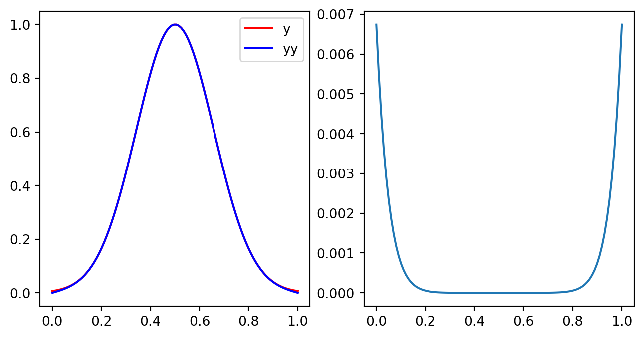
Show the code
y_r = lambda x, t: (1.0/np.sqrt(1+80*t)*(np.exp(-20*(x-0.5)**2/(1.0+80*t)) - np.exp(-20*(x-1.5)**2/(1.0+80.0*t))-np.exp(-20*(x+0.5)**2/(1.0+80.0*t))))


t_end = 0.1
t_step = 10000
times = np.linspace(0, t_end, t_step + 1)
dt = times[1] - times[0]
dx = x[1] - x[0]
rr = dt / dx**2.0
yrr = y_r(x, t_end)

y_solve = np.zeros([len(x), t_step + 1])
y_solve[:, 0] = yy(x)
source = np.zeros(x.shape)


def explicit_parabolic(x, y_solve, rr, dt, source):
    for nn in range(t_step):
        for i in range(1, len(x)-1):
            y_solve[i,nn+1]=rr*y_solve[i+1,nn]+(1-2*rr)*y_solve[i,nn]+rr*y_solve[i-1,nn] + dt * source[i]


explicit_parabolic(x, y_solve, rr, dt, source)
for i in range(0, t_step+1, 2000):
    plt.plot(x, y_solve[:, i], lw = 5, label = str(i))
plt.plot(x, yrr, 'b-.', lw = 3, label = 'accurate')
plt.legend()
plt.title('r = ' + str(rr))
plt.show()


t_end = 0.1
t_step = 1000
times = np.linspace(0, t_end, t_step + 1)
dt = times[1] - times[0]
dx = x[1] - x[0]
rr = dt / dx**2.0
yrr = y_r(x, t_end)

y_solve = np.zeros([len(x), t_step + 1])
y_solve[:, 0] = yy(x)

source = np.zeros(x.shape)
explicit_parabolic(x, y_solve, rr, dt, source)

for i in range(0, t_step+1, 200):
    plt.plot(x, y_solve[:, i], lw = 5, label = str(i))
plt.plot(x, yrr, 'b-.', lw = 3, label = 'accurate')
plt.legend()
plt.title('r = ' + str(rr))
plt.show()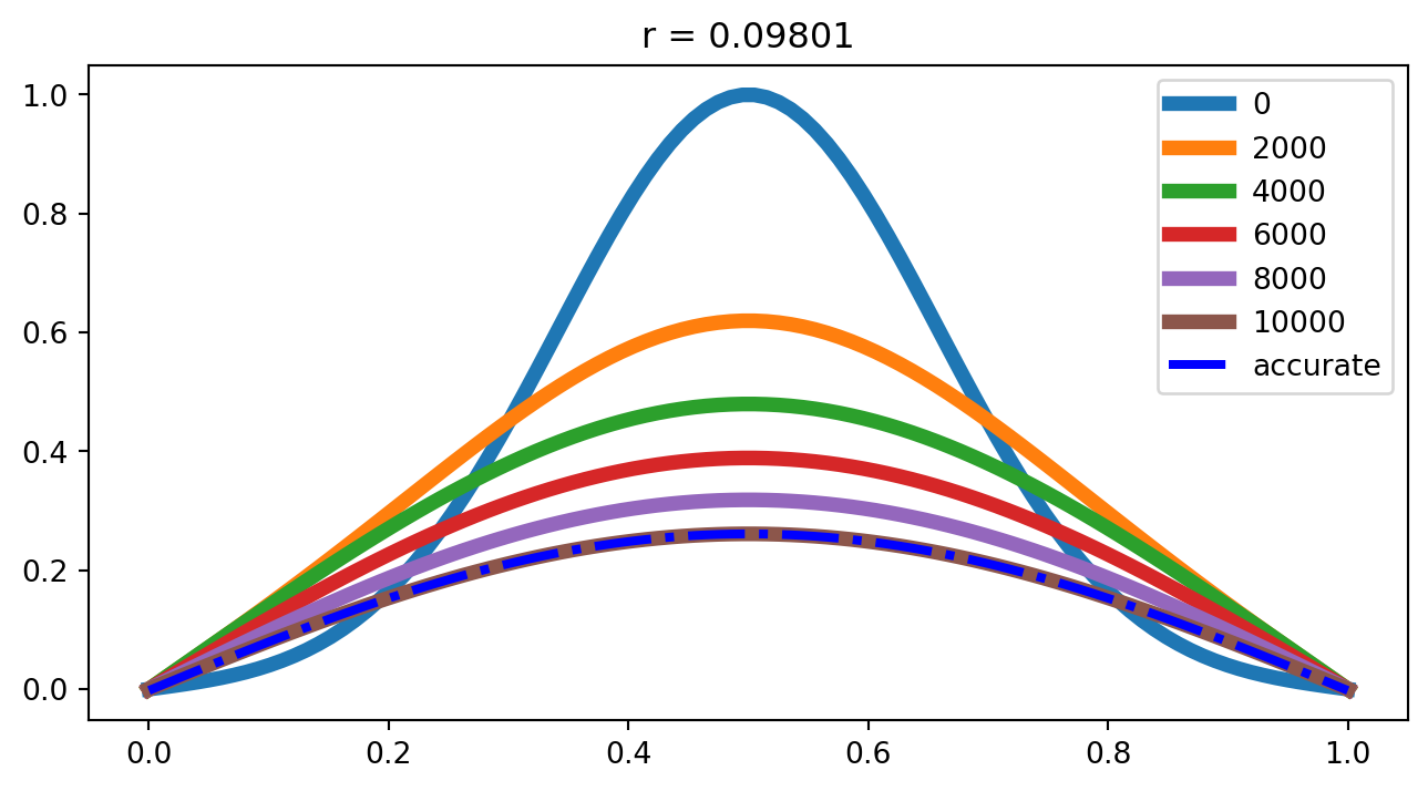
/var/folders/r_/ctnsy93118b_yw2h5rqqpmxh0000gn/T/ipykernel_3224/665637868.py:20: RuntimeWarning:

overflow encountered in scalar add

出现这一情况的原因是因为前述显式差分格式是一个条件稳定格式,只有当满足下式时才是稳定的。
\[ \frac{\Delta t}{h^2} \leq \frac{1}{2} \]
当我们选用更小的空间步长\(h\)时,迫使我们不得不取一个更小的时间步长 \(\Delta t\) ,这将付出很大的代价,特别是这个时间步长比恰当地描述系统演化所需要的自然时间尺度要小的多时。
- 《计算物理学》 复旦大学,顾长鑫 P108.
- 《偏微分方程数值解法》 陆金甫 P82.
对一维热传导方程 \(u_t = a^2 u_{xx}\)
取 \(x = i\Delta x, ~~ t = j\Delta t, ~~ i = 0, 1, ..., N; ~~ j = 0,1,2...\)
let \(r = \frac{\Delta t}{(\Delta x)^2}a^2\)
显式差分公式 \(u_i^{j+1} = (1-2r)u_i^j + r(u_{i+1}^j + u_{i-1}^j)\)
稳定条件: \[ r = \frac{\Delta t}{(\Delta x)^2}a^2 < \frac{1}{2} \tag{14}\]
Example 10 以有限长细杆的热传导问题为例,定解问题是
\(l = 20, ~~ t = 25, ~~ a^2 = 1, ~~ \phi(x) = \left\lbrace \begin{matrix*}[l] 1, ~~ (10 \leq x \leq 11) \\ 0, ~~(x < 10, x > 11) \end{matrix*} \right.\)
%filename: chapter4_example_10.m
clear all
close all
clc
%example-10;
L=20;T=25;A=1;
h=0.5;
N=L/h;
x=0:h:L;
delta_t=0.05;
N_t=T/delta_t;
t=0:delta_t:T;
[XX,TT]=meshgrid(x,t);
y=zeros(length(x),length(t));
y((10/h+1):(11/h+1),1)=1; %初值条件

rr=delta_t/h^2*A

for j=1:N_t    %时间上的步数
    for i=2:N   %空间上的点
        y(i,j+1)=rr*y(i+1,j)+(1-2*rr)*y(i,j)+rr*y(i-1,j);
    end
end

figure; plot(x,y(:,N_t+1)) %终了时刻杆上的温度分布
xlabel('x'),ylabel('u')
figure; surf(XX,TT,y')
xlabel('x'),ylabel('t'),zlabel('u')
figure; contourf(XX,TT,y')
xlabel('x'),ylabel('t')
colorbar
Show the code
x = np.linspace(0, 20, 500)
t_end = 25.0
t_step = 100000
times = np.linspace(0, t_end, t_step + 1)
dt = times[1] - times[0]
dx = x[1] - x[0]
rr = dt / dx**2.0

print('r = ', rr)
y_solve = np.zeros([len(x), t_step + 1])
for i in range(len(x)):
    if x[i] >= 10 and x[i] <= 11:
        y_solve[i, 0] = 1.0

source = np.zeros(x.shape)
explicit_parabolic(x, y_solve, rr, dt, source)

fig = plt.figure(figsize = (10, 4))
ax = fig.add_subplot(121, projection='3d')
X, Y = np.meshgrid(times, x)

ax.plot_surface(X, Y, y_solve, cmap = 'jet')

ax.set_xlabel(r'$t$')
ax.set_ylabel(r'$x$')
ax.set_zlabel(r'$\Phi$')

plt.subplot(122)
plt.imshow(y_solve, cmap = 'jet', aspect='auto')
plt.colorbar()
plt.show()
r = 0.15562562500000002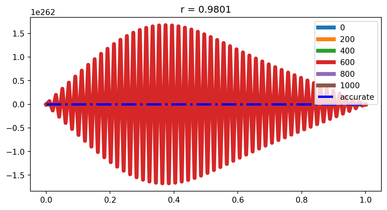
3.1 隐式差分格式
Refer (Equation 11) 将空间的二阶导数用新时刻上的三点差分公式来近似代替 \[
\frac{\Phi_i^{n+1} - \Phi_i^n}{\Delta t} = \frac{1}{h^2}(\Phi_{i+1}^{n+1} - 2\Phi_i^{n+1} + \Phi_{i-1}^{n+1}) + S_i^n
\]
此格式的截断误差为\(O(h^2, \Delta t)\),它是无条件稳定的,即对于任何步长都是稳定的,因此可以用大的时间步长。 \[ \Phi_i^{n+1} = \Phi_i^n + \frac{\Delta t}{h^2}(\Phi_{i+1}^{n+1} - 2\Phi_i^{n+1} + \Phi_{i-1}^{n+1}) + S_i^n\Delta t \tag{15}\]
\[
\xrightarrow{ r = \Delta t /h^2} ~~~ -r \Phi_{i - 1}^{n+1} + (1 + 2r) \Phi_i^{n+1} - r\Phi_{i+1}^{n+1} = \Phi_i^n + S_i^n\Delta t
\tag{16}\] 对于已知边界条件的情况,可将上述方程组写成
Example 11 (用隐式差分格式计算例9) Refer (Equation 11, Equation 5, Equation 12, Equation 13) Equation 16
对于下述隐式差分格式,考虑\(S=0\)并且边界条件\(\Phi (0) = \Phi (1)=0\)
\[ \begin{pmatrix} 1+2r & -r \\ -r & 1+2r & -r \\ &\ddots & \ddots & \ddots \\ & & -r & 1+2r & -r & \\ & & & -r & 1+2r \\ \end{pmatrix} \begin{pmatrix} \Phi_1^{n+1} \\ \Phi_2^{n+1} \\ \vdots \\ \Phi_{N-2}^{n+1} \\ \Phi_{N-1}^{n+1} \end{pmatrix} = \begin{pmatrix} \Phi_1^{n} \\ \Phi_2^{n} \\ \vdots \\ \Phi_{N-2}^{n} \\ \Phi_{N-1}^{n+1} \end{pmatrix} \]
Code:
%filename: chapter4_example_11_yinshichafen.m
clear all
close all
clc
%for example-11,用隐式差分格式求解抛物型偏微分方程

N=1000;
h=1/N;
x=0:h:1;    %空间步长
y=@(x) exp(-20*(x-0.5).^2)-exp(-20*(x-1.5).^2)-exp(-20*(x+0.5).^2); %初始条件

delta_t=0.0001; %时间步长
t=0:delta_t:0.1;%时间上的迭代次数,决定了最终得到哪个时刻的解
y_n=zeros(N+1,length(t));
y_n(1,1)=0;  %边界条件
y_n(N+1,1)=0; %边界条件
%yy=zeros(2:N,1);

%精确解
y_r=@(xx,t)(1/sqrt(1+80*t).*(exp(-20*(xx-0.5).^2/(1+80*t))...
    -exp(-20*(xx-1.5).^2/(1+80*t))-exp(-20*(xx+0.5).^2/(1+80*t))));

%================数值解(隐式差分格式)==========================
rr=delta_t/h^2

A=zeros(N-1,N-1); %给系数矩阵赋值
A(1,1)=1+2*rr; A(1,2)=-rr; %将系数矩阵第一行和最后一行单独赋值
A(N-1,N-1)=1+2*rr; A(N-1,N-2)=-rr;
for i=2:N-2       %对系数矩阵中中间行赋值
    A(i,i)=1+2*rr;
    A(i,i-1)=-rr;
    A(i,i+1)=-rr;
end
B(1:N-1,1)=y(h:h:(N-1)*h);

AA=A^-1; %矩阵求逆
yy=zeros(N-1,1);
for ii=1:length(t)-1
%给方程右边的列矩阵赋值
yy=AA*B;   %采用矩阵乘法获得解的列矩阵
B=yy;
%获得新的方程右边的列矩阵的值,对于此特殊问题,S=0,边值为0,B与yy相等,但不具有普遍性
%y_n(N+1,i)=yy;
end

y_n(2:N,length(t))=yy(1:N-1,1);
%注意解析结果的最后一个值不为0
error=y_n(:,length(t))-y_r(x,delta_t*(length(t)-1))';
%注意:y_(:,length(t))以列存储,y_r(x,delta_t*N_t)以行数组存储,所以需要转置运算
figure(1),plot(x,y_n(:,length(t)),'-r',x,y_r(x,delta_t*(length(t)-1)),'b',x,y(x),'-k')
legend('数值结果','解析结果','初始状态')
figure(2),plot(x,error)
legend('数值结果与解析结果间的误差')
Show the code
x = np.linspace(0, 1, 101)
yy = lambda x: (np.exp(-20*(x-0.5)**2)-np.exp(-20*(x-1.5)**2)-np.exp(-20*(x+0.5)**2))

y_r = lambda x, t: (1.0/np.sqrt(1+80*t)*(np.exp(-20*(x-0.5)**2/(1.0+80*t)) - np.exp(-20*(x-1.5)**2/(1.0+80.0*t))-np.exp(-20*(x+0.5)**2/(1.0+80.0*t))))

t_end = 0.1
t_step = 100
times = np.linspace(0, t_end, t_step + 1)
dt = times[1] - times[0]
dx = x[1] - x[0]
rr = dt / dx**2.0
yrr = y_r(x, t_end)

y_solve = np.zeros([len(x), t_step + 1])
y_solve[:, 0] = yy(x)

def implicit_parabolic(x, y_solve, rr, dt, source):
    imat = np.eye(len(x) - 2) * (1 + 2.0 * rr)
    for i in range(len(x) - 3):
        imat[i, i + 1] = -rr
        imat[i + 1, i] = -rr
    iimat = np.linalg.inv(imat)
    for nn in range(t_step):
        temp = y_solve[1:-1, nn] + source[1:-1] * dt
        temp[0] = temp[0] + rr*y_solve[0, nn+1]
        temp[-1] = temp[-1] + rr*y_solve[-1, nn+1]
        y_solve[1:-1, nn + 1] = np.dot(iimat, temp)

source = np.zeros(x.shape)
implicit_parabolic(x, y_solve, rr, dt, source)
for i in range(0, t_step + 1, 20):
    plt.plot(x, y_solve[:, i], lw = 5, label = 't = ' + str(times[i]))
plt.plot(x, y_solve[:, -1], lw = 5, color = 'red', label = 'implicit')
plt.plot(x, yrr, 'b-.', lw = 3, label = 'accurate')
plt.legend()
plt.title('r = ' + str(rr))
plt.show()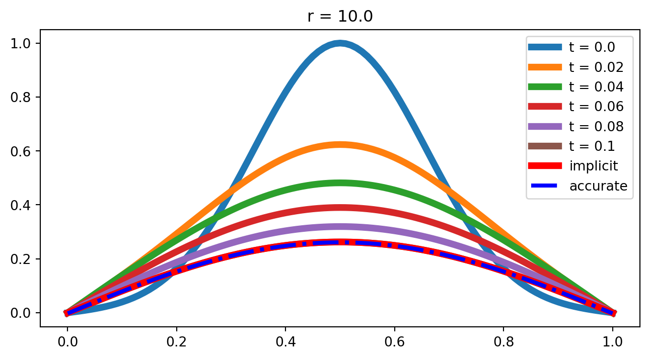
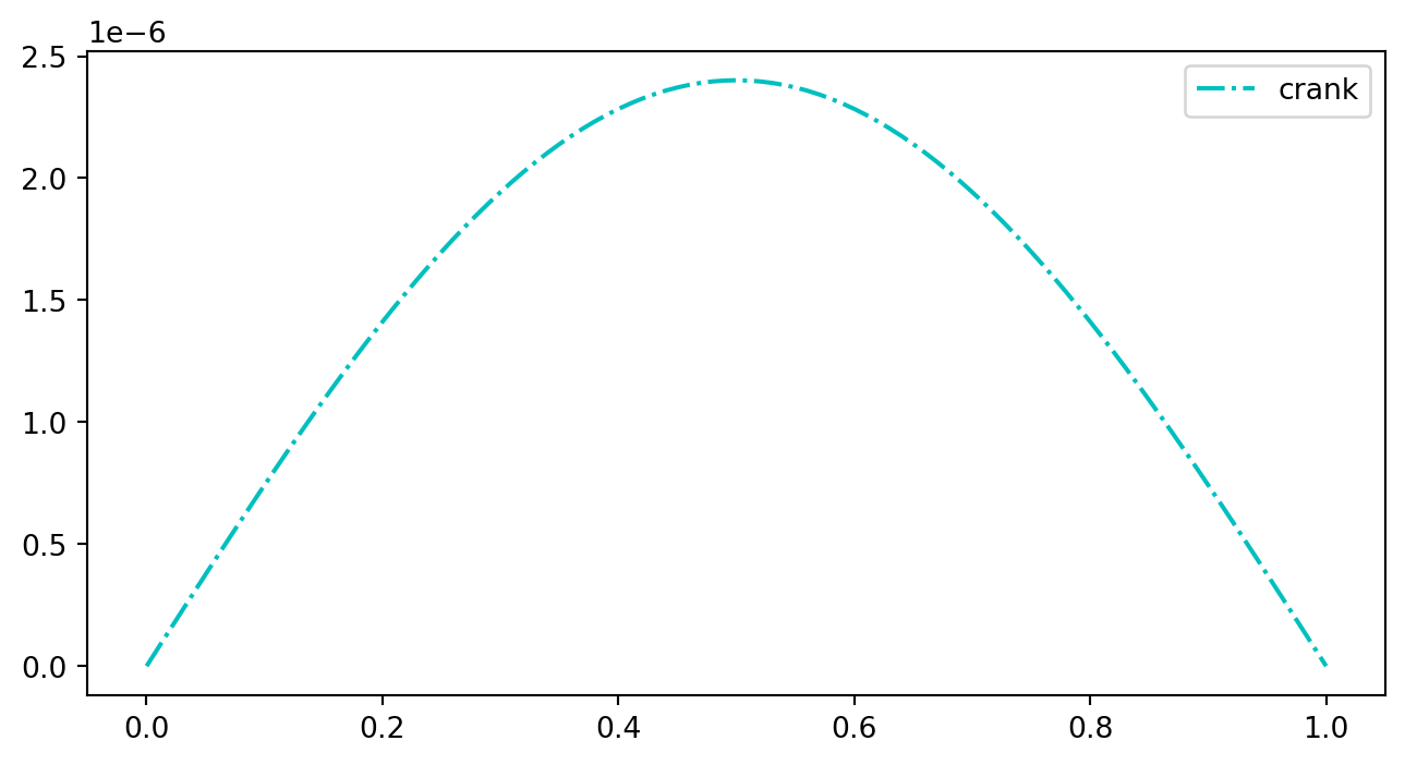
3.2 平均隐式差分格式 (Crank–Nicolson方法)
三点隐式差分公式 \[
\frac{\Phi_i^{n+1} - \Phi_i^n}{\Delta t} = \frac{1}{h^2}(\Phi_{i+1}^{n+1} - 2\Phi_i^{n+1} + \Phi_{i-1}^{n+1}) +S_i^n
\] 若将空间的二阶导数用新旧时刻上的三点差分公式的平均值来近似代替 \[
\frac{\Phi_i^{n+1} - \Phi_i^n}{\Delta t} = \frac{1}{2h^2}[(\Phi_{i+1}^{n+1} - 2\Phi_i^{n+1} + \Phi_{i-1}^{n+1}) + (\Phi_{i+1}^{n} - 2\Phi_i^{n} + \Phi_{i-1}^{n})]+S_i^n
\] 此为六点隐式差分公式,此格式的截断误差为\(O(h^2,\Delta t^2)\),它也是无条件稳定的,即对于任何步长都是稳定的。其
潜在的缺点: 对时间每进行一次计算都需要解一个线性方程组以求 \(\Phi_{n+1}\) ,但我们可以看到,对于给定值r,系数矩阵不变,因此可以直接左乘其逆矩阵。
Example 11-1 以有限长细杆的热传导问题为例,定解问题是 \[ \left\lbrace \begin{matrix*}[l] u_t = a^2u_{xx}, ~~ 0\leq x \leq 1, ~t>0 \\ u(0, t) = 0, ~~ u(1, t) = 0 \\ u(x, t = 0) = \sin \pi x \end{matrix*} \right. \]
取\(a = 1\),利用分离变量法可得上述方程的解析解为 \[
u(x, t) = e^{-\pi^2 t} \sin\pi x, ~~ 0 \leq x \leq 1, ~~ t\geq 0
\] 分别用
Refer: (Equation 9)
Explicit: (Equation 11)
implicit: (Equation 16) (Equation 17)
avg implicit: (Equation 18) (Equation 19)
Code:
%filename: chapter4_example_11_1_xianshi_yinshi_pingjun.m
clear all
close all
clc
%for example-11-1,分别用显示差分格式,隐式差分格式和
%平均隐式差分格式求解抛物型偏微分方程;
format long
N=100;h=1/N;
x=0:h:1;          %空间步长
u=@(x) sin(pi*x); %初始条件
T=0.4;            %要求时刻
delta_t=0.0025;   %时间步长
t=0:delta_t:T;
%===========精确解============================
u_r=@(x,t)exp(-pi^2*t).*sin(pi*x);
%===========数值解(显示差分格式)============
N_t=T/delta_t;     %时间上的迭代次数,决定了最终得到哪个时刻的解
u_1=zeros(N+1,N_t+1); %显示差分格式结果
u_1(1,1)=0;  %边界条件,可以注释掉
u_1(N+1,1)=0; %边界条件,可以注释掉
u_1(2:N,1)=u(h:h:(N-1)*h); %给u_1数组赋初值,注意u是采用句柄函数定义的
rr=delta_t/h^2
for j=1:N_t    %时间上的步数
    for i=2:N   %空间上的点
        u_1(i,j+1)=rr*(u_1(i+1,j)+u_1(i-1,j))+(1-2*rr)*u_1(i,j);
    end
end
%================数值解(隐式差分格式)==========================
A=zeros(N-1,N-1); %给系数矩阵赋值
A(1,1)=1+2*rr; A(1,2)=-rr; %将系数矩阵第一行和最后一行单独赋值
A(N-1,N-1)=1+2*rr; A(N-1,N-2)=-rr;
for i=2:N-2       %对系数矩阵中中间行赋值
    A(i,i)=1+2*rr;
    A(i,i-1)=-rr;
    A(i,i+1)=-rr;
end
B=zeros(N-1,1);
B(1:N-1,1)=u(h:h:(N-1)*h); %
AA=A^-1;
yy=zeros(N-1,1);
u_2=zeros(N+1,N_t+1); %隐式差分格式结果
for ii=1:N_t
%给方程右边的列矩阵赋值
yy=AA*B;   %采用矩阵乘法获得解得列矩阵
B=yy;
%获得新的方程右边的列矩阵的值,对于此特殊问题,S=0,边值为0,B与yy相等,但不具有普遍性
u_2(2:N,ii+1)=yy;
end

%================数值解(平均隐式差分格式)==========================
A_1=zeros(N-1,N-1); %给系数矩阵赋值
A_1(1,1)=1+rr; A_1(1,2)=-rr/2; %将系数矩阵第一行和最后一行单独赋值
A_1(N-1,N-1)=1+rr; A_1(N-1,N-2)=-rr/2;
for i=2:N-2       %对系数矩阵中中间行赋值
    A_1(i,i)=1+rr;
    A_1(i,i-1)=-rr/2;
    A_1(i,i+1)=-rr/2;
end
B_1=zeros(N-1,1);
B_1(1:N-1,1)=0.5*rr*u(2*h:h:N*h)+(1-rr)*u(h:h:(N-1)*h)+0.5*rr*u(0:h:(N-2)*h); %

AA_1=A_1^-1;              %矩阵求逆
yy=zeros(N-1,1);
u_3=zeros(N+1,N_t+1); %平均隐式差分格式结果
for ii=1:N_t
%给方程右边的列矩阵赋值
yy=AA_1*B_1;   %采用矩阵除法获得解得列矩阵
u_3(2:N,ii+1)=yy(1:N-1,1);
B_1(1:N-1,1)=0.5*rr*u_3(3:N+1,ii+1)+(1-rr)*u_3(2:N,ii+1)+0.5*rr*u_3(1:N-1,ii+1); %
%获得新的方程右边的列矩阵的值
end
u_1(round(0.4/h)+1,N_t+1) %三种不同方法求得的u(0.4,0.4)
u_2(round(0.4/h)+1,N_t+1)
u_3(round(0.4/h)+1,N_t+1)

error_1=u_1(:,N_t+1)-u_r(x,delta_t*N_t)';
error_2=u_2(:,N_t+1)-u_r(x,delta_t*N_t)';
error_3=u_3(:,N_t+1)-u_r(x,delta_t*N_t)';
%注意:u_1(:,N_t+1)以列存储,u_r(x,delta_t*N_t)以行数组存储,所以需要转置运算
figure(1),plot(x,u_1(:,N_t+1),'-*r',x,u_r(x,delta_t*N_t),'b')
figure(2),plot(x,u_2(:,N_t+1),'-*g',x,u_r(x,delta_t*N_t),'b')
figure(3),plot(x,u_3(:,N_t+1),'-*k',x,u_r(x,delta_t*N_t),'b')
figure(4),plot(x,error_1,'r')
figure(5),plot(x,error_2,'k')
figure(6),plot(x,error_3,'b')
figure(7),plot(x,u_1(:,N_t+1),'k',x,u_2(:,N_t+1),'-r',x,u_3(:,N_t+1),'-g',x,u_r(x,delta_t*N_t),'b')
legend('数值结果-显式差分','数值结果-隐式差分','数值结果-平均隐式差分','解析结果')
%legend('数值结果-显式差分的误差','数值结果-隐式差分的误差','数值结果-平均隐式差分的误差')
Show the code
def avg_implicit_parabolic(x, y_solve, rr, dt, source):
imat = np.eye(len(x) - 2) * (1 + rr)
for i in range(len(x) - 3):
imat[i, i + 1] = -0.5 * rr
imat[i + 1, i] = -0.5 * rr
iimat = np.linalg.inv(imat)
for nn in range(t_step):
temp = 0.5 * rr * y_solve[2:, nn] + (1 - rr) * y_solve[1:-1, nn] + 0.5 * rr * y_solve[0:-2, nn] + source[1:-1] * dt
temp[0] = temp[0] + 0.5 * rr * y_solve[0, nn+1]
temp[-1] = temp[-1] + 0.5 * rr*y_solve[-1, nn+1]
y_solve[1:-1, nn + 1] = np.dot(iimat, temp)
x = np.linspace(0, 1, 101)
yy = lambda x: np.sin(np.pi * x)
y_r = lambda x, t: np.exp(-np.pi**2*t)*np.sin(np.pi*x)
t_end = 0.4
t_step = int(t_end / 0.0025)
times = np.linspace(0, t_end, t_step + 1)
dt = times[1] - times[0]
dx = x[1] - x[0]
rr = dt / dx**2.0
yrr = y_r(x, t_end)
y_solve = np.zeros([len(x), t_step + 1])
y_solve[:, 0] = yy(x)
y_solve[0, 0] = 0.0
y_solve[-1, 0] = 0.0
y_solve2 = y_solve.copy()
y_solve0 = y_solve.copy()
source = np.zeros(x.shape)
avg_implicit_parabolic(x, y_solve2, rr, dt, source)
implicit_parabolic(x, y_solve, rr, dt, source)
explicit_parabolic(x, y_solve0, rr, dt, source)
#plt.plot(x, y_solve0[:, -1], 'r-', label = 'explicit')
plt.plot(x, y_solve[:, -1], 'b-', label = 'implicit')
plt.plot(x, y_solve2[:, -1], 'c-.', label = 'avg')
#plt.plot(x, yrr, 'k', lw = 3, label = 'accurate')
plt.legend()
plt.title('r = ' + str(rr))
plt.show()
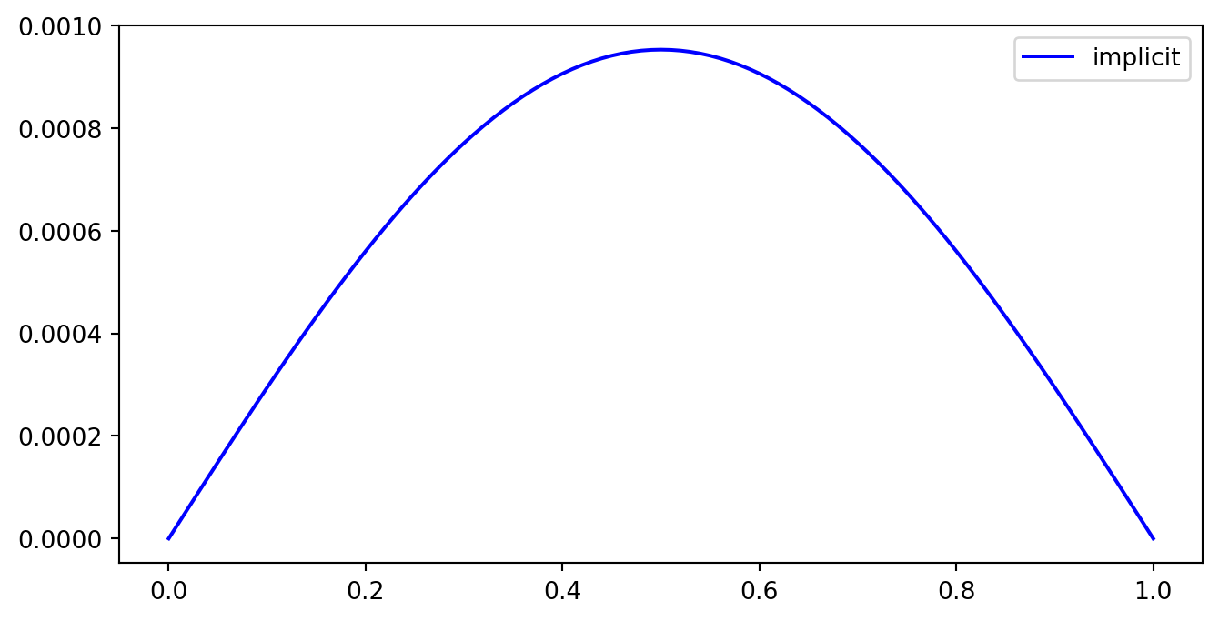
#plt.plot(x, y_solve0[:, -1] - yrr, 'r-', label = 'explicit')
plt.plot(x, y_solve[:, -1] - yrr, 'b-', label = 'implicit')
plt.legend()
plt.show()
plt.plot(x, y_solve2[:, -1] - yrr, 'c-.', label = 'crank')
plt.legend()
plt.show()
4 隐式差分格式的算符表示
Refer (Equation 10) 将空间的二阶导数用新时刻上的三点差分公式来近似代替 \[ \frac{\Phi_i^{n+1} - \Phi_{i}^{n}}{\Delta t} = \frac{1}{h^2}(\delta^2 \Phi^{n+1})_i + S_i^n \tag{20}\] 引入算符\(H\),使得 \[ H\Phi_i^{n+1} = -\frac{1}{h^2}(\Phi_{i+1}^{n+1} - 2\Phi_i^{n+1} + \Phi_{i-1}^{n+1}) = -\frac{1}{h^2}(\delta^2\Phi^{n+1})_i \] with (Equation 20)
\[ \Phi_i^{n+1} = \frac{1}{1+H\Delta t}[\Phi_i^n + S_i^n \Delta t] \tag{21}\]
平均隐式差分格式 (Crank–Nicolson方法)的算符表示 \[ \frac{\Phi_i^{n+1} - \Phi_{i}^{n}}{\Delta t} = \frac{1}{h^2}\left(\delta^2 [\Phi^{n+1} + \Phi^{n}]\right)_i + S_i^n \]
\[ \Longrightarrow \frac{\Phi_i^{n+1} - \Phi_{i}^{n}}{\Delta t} = -\frac{1}{h^2}H\Phi^{n+1}_i -\frac{1}{h^2}H\Phi^{n}_i + S_i^n \]
\[ \Longrightarrow \Phi_i^{n+1} = \frac{1}{1+\frac{1}{2}H\Delta t}\left[ \left( 1- \frac{1}{2}H\Delta t \right)\Phi_i^n + S_i^n\Delta t \right] \]
\[ \Longrightarrow \Phi_i^{n+1} = \frac{1}{1+\frac{1}{2}H\Delta t}\left[ \left( 1- \frac{1}{2}H\Delta t \right)\Phi_i^n + S_i^n\Delta t \right] \]
4.1 含时薛定谔方程
Refer (Note 1)
一维运动粒子贯穿势垒的薛定谔方程 \[ i\hbar \phi_t = -\frac{\hbar^2}{2m}\nabla^2 \phi + V\phi \] 令\(\hbar=1,2m=1\),一维方程可化为 \[ \phi_t = i(\partial_{xx} - V)\phi \equiv -iH\phi \] with \[ H\phi_i^n = -\frac{1}{h^2}\left( \phi_{i+1}^n - 2\phi_i^n + \phi_{i-1}^n \right) + V_i \phi_i^n \tag{22}\] averaged difference: \[ \phi^{n+1} = \left(\frac{1-i\frac{1}{2}H\Delta t}{1+i\frac{1}{2}H\Delta t}\right)\phi^n;~~~~~ H = -\partial_{xx} + V \] 可以证明这个递归关系是幺正的(\(UU^\dagger=1\)),即保证波函数的模方在全空间的积分不随时间变化,这正是量子力学所要求的。 \[ \phi^{n+1} = \left(\frac{1-i\frac{1}{2}H\Delta t}{1+i\frac{1}{2}H\Delta t}\right)\phi^n \leftrightarrow \phi^{n+1} = e^{-iH\Delta t}\phi^n\] 量子力学中的哈密顿算符 \(H = \frac{P^2}{2m} + V = \frac{(i\hbar\nabla)^2}{2m} + V = -\frac{\hbar^2}{2m}\partial_{xx} + V\) let \(\hbar = 1, 2m = 1\)
实际的数值计算中 \[ \phi^{n+1} = \left( \frac{2}{1+i\frac{1}{2}H\Delta t} -1\right)\phi^n \equiv \chi - \phi^n ~~~~~ \text{with} ~~ \chi = \frac{2\phi^n}{1+i\frac{1}{2}H\Delta t} \] 为了在每一个时间步求出中间函数\(\chi\),显式的写出其满足的差分方程 \[ \chi = \frac{2\phi^n}{1+i\frac{1}{2}H\Delta t} \Longrightarrow \left(1+i\frac{\Delta t}{2}H\right)\chi = 2\phi^n \] Refer (Equation 22) \[ \left(1+i\frac{\Delta t}{2}V_j\right)\chi_j - i\frac{\Delta t}{2}\frac{\chi_{j+1} - 2\chi_j + \chi_{j-1}}{h^2} = 2\phi_j^n \] \[ \Longrightarrow ~~ \frac{\Delta t}{2ih^2}\left[\left(\frac{2ih^2}{\Delta t} - h^2V_j - 2 \right)\chi_j + \chi_{j+1} + \chi_{j-1} \right] = 2\phi_j^n \] \[ \Longrightarrow \chi_{j-1} + \left[-2 + \frac{2ih^2}{\Delta t} -h^2V_j\right]\chi_j + \chi_{j+1} = \frac{4ih^2}{\Delta t}\phi_j^n, ~~j=1,2,...,N-1 \] 上述方程组可以写成矩阵形式,用矩阵求逆法可获得方程组的解。 let \(-2 + \frac{2ih^2}{\Delta t} -h^2V_j = r\) \[ \begin{pmatrix} r & 1 \\ 1 & r & 1 \\ & \ddots & \ddots & \ddots \\ & & & 1 & r & 1 \\ & & & & 1 & r \\ \end{pmatrix} \begin{pmatrix} \chi_1 \\ \chi_2 \\ \vdots \\ \chi_{N-2} \\ \chi_{N-1} \end{pmatrix} = \begin{pmatrix} \frac{4ih^2}{\Delta t}\phi_1^n - \chi_0 \\ \frac{4ih^2}{\Delta t}\phi_2^n \\ \vdots \\ \frac{4ih^2}{\Delta t}\phi_{N-2}^n \\ \frac{4ih^2}{\Delta t}\phi_{N-1}^n + \chi_N \end{pmatrix} \]
Example 12 \(220\)个点; 方势垒,\(V=0.18, [105, 115]\); 初始波包为Guass波包,平均波数为\(k_0=0.6, \sigma=10\),中心位于编号为\(40\)的格子; 时间步长\(=1\),演化时间\(130\)
初始波包为Guass波包 \[ \Psi(x, 0) = e^{ik_0x}\cdot e^{-\frac{(x-x_0)^2\log_{10}2}{\sigma^2}} \] Code:
%filename: chapter4_example_12_schrodinger_td.m
clear all
close all
clc
%数值求解含时薛定谔方程,研究波函数在遇到势垒后的行为

NPTS=220;           %格点数
sigma=10;k0=0.6;    %Gauss波包参数
x0=40;              %Gauss波包参数
time=400;           %演化时间,可以用更长演化时间观测波包运动
N=NPTS-1;            %空间被离散成NPTS-1段
v(1,NPTS)=0;        %格点上的势函数V
v(1,105:115)=-12.0;   %势垒,可改变势垒高度,观察波函数穿越势垒的情况
%注意在下面的矩阵中,空间步长h=1,时间步长delta_t=1,
%系数矩阵求法见ppt中标注为(2)的公式
%A=diag(-2+2i-v(2:N),0)+diag(ones(N-2,1),1)+diag(ones(N-2,1),-1);  %系数矩阵
%使用diag函数可以使程序大大简化
A=zeros(N-1,N-1);
A(1,1)=-2+2i-v(1,2);
A(1,2)=1;
A(N-1,N-1)=-2+2i-v(1,N);
A(N-1,N-2)=1;
for n=2:N-2
    A(n,n)=-2+2i-v(1,n+1);
    A(n,n+1)=1;
    A(n,n-1)=1;
end
PHI0(1)=0;PHI0(NPTS)=0;  %边界条件
for x=2:NPTS-1;
PHI0(x)=exp(k0*i*x)*exp(-(x-x0)^2*log10(2)/sigma^2); %初始波函数,Gauss波包
end
PHI=zeros(NPTS,time);
PHI(:,1)=PHI0';
for y=2:time
CHI(2:NPTS-1,y)=4i*(A\PHI(2:NPTS-1,y-1));  %见公式(2),步长h和时间间隔delta_t都为1
PHI(2:NPTS-1,y)=CHI(2:NPTS-1,y)-PHI(2:NPTS-1,y-1);%见公式(1)
end
mo=moviein(time);
for j=1:time
plot([1:NPTS],abs(PHI(:,j)).^2/norm(PHI(:,j)).^2,'r',[1:NPTS],v,'b');
%画波函数时我们做了归一化处理,norm为取模运算
axis([0,220,0,0.1]);
mo(j)=getframe; %对当前图形拍照后产生的数据向量依次存放于画面构架数组中
end
movie(mo,1,50)  %以每秒50帧的速度,重复播放1次

figure;plot([1:NPTS],abs(PHI(:,1)).^2/norm(PHI(:,1)).^2,'r',[1:NPTS],v,'b')
%初始波包5 双曲型偏微分方程
5.1 一阶双曲型方程的差分格式
考虑一阶双曲型方程的初值问题: \[ \left\lbrace \begin{matrix*}[l] u_t + au_x = 0, ~~~~ t>0,-\infty < x < + \infty \\ u(x, 0) = \phi(x), ~~~ -\infty < x < + \infty \end{matrix*} \right. \] 将\(x-t\)平面分割成矩形网格,取\(x\)方向的步长为\(h, t\)方向的步长为\(\tau\),网格线为$x=ih, i=0, , ,…; t=j, j=0,1,2,… $
以不同的差分近似偏导数,可以得到如下差分格式:
\[ \frac{u_i^{j+1} - u_i^j}{\tau} + a \frac{u_{i+1}^j - u_i^j}{h} = 0 \]
空间向前差分(右偏心格式)
\[
\frac{u_i^{j+1} - u_i^j}{\tau} + a \frac{u_{i}^j - u_{i-1}^j}{h} = 0
\] >
\[
\frac{u_i^{j+1} - u_i^j}{\tau} + a \frac{u_{i+1}^j - u_{i-1}^j}{2h} = 0
\] >
截断误差分别为\(O(\tau + h), O(\tau + h)\)与\(O(\tau + h^2)\),上述三式可以写为
\[ u_i^{j+1} = u_i^j - \frac{a\tau}{h}(u_{i+1}^j - u_{i}^j) \tag{23}\]
\[ u_i^{j+1} = u_i^j - \frac{a\tau}{h}(u_{i}^j - u_{i-1}^j) \tag{24}\]
\[ u_i^{j+1} = u_i^j - \frac{a\tau}{2h}(u_{i+1}^j - u_{i-1}^j) \tag{25}\]
它们都是显式差分格式。从稳定性分析将会知道,这三格式并不都可用。
- 当a>0时,
- 显式差分格式(Equation 23)是绝对不稳定的;
- 显式差分格式(Equation 24)是条件稳定的,稳定条件为\(\frac{a\tau}{h}\leq 1\);
- 显式差分格式(Equation 25)也是绝对不稳定的;
- 当a<0时,
- 显式差分格式(Equation 23)是条件稳定的,稳定条件为\(\frac{|a|\tau}{h} \leq 1\)
- 显式差分格式(Equation 24)是绝对不稳定的;
- 显式差分格式(Equation 25)是绝对不稳定的;
\[
\left\lbrace
\begin{matrix*}[l]
u_i^{j+1} = u_i^j - \frac{a\tau}{h}(u_{i+1}^j - u_{i}^j); ~~ (a>0, \frac{a\tau}{h} \leq 1) \\
u_i^{j+1} = u_i^j - \frac{a\tau}{h}(u_{i}^j - u_{i-1}^j); ~~(a<0, \frac{|a|\tau}{h} \leq 1)
\end{matrix*}
\right.
\] 上式称作双曲型偏微分方程数值求解的
5.2 二阶双曲型方程的差分格式
\[ \Phi_{tt} = \Delta \Phi \] 弦振动方程与时变电磁场中的波动方程都是一维(二阶)双曲型方程的典型例子。
两端固定的弦,相应的运动方程为 \(u_{tt} = a^2u_{xx}\).
\[ \Longrightarrow u_i^{j+1} = c(u_{i+1}^j + u_{i-1}^j) + 2(1-c)u_i^j - u_i^{j-1}; ~~~ c = a^2\frac{\Delta t^2}{\Delta x^2} \]
- 当\(c\leq1\)时,上述差分格式是稳定的;
- 当\(c>1\)时则是不稳定的。此格式的截断误差为\(O(h^2,\Delta t^2)\)。
- 《计算物理学》 复旦大学,顾长鑫 P104.
- 《偏微分方程数值解法》 陆金甫 P61-63.
显式公式表明,需要两行已知的数据才能求出下一行的数值。 
5.2.1 利用初始条件获得公式计算的启动值
设\(t=0\)时对应\(j=1\),初始位移\(j(x)\)和初始速度\(y(x)\)离散化以后得\(j_i =j(x_i)\)和\(y_i= y(x_i)\)。
初始位移\(u_i^1 = \phi_i\)
初始速度用中心差分可表示为: \(\frac{\partial u_i^1}{\partial t} = \frac{u_i^2 - u_i^0}{2\Delta t} = \psi_i\) \[ u_i^0 = u_i^2 - 2\Delta t \psi_i \] 将其带入下式(\(j=1\)) \[ u_i^{j+1} = c(u_{i+1}^j + u_{i-1}^j) + 2(1-c)u_i^j - u_i^{j-1} \] \[ \Longrightarrow u_i^2 = \frac{c}{2}(u_{i+1}^1 + u_{i-1}^1) + (1-c)u_i^1 + \psi_i\Delta t \] 更简单的是,初始速度用向前差分表示 \[ \psi_i = \frac{u_i^2 - u_i^1}{\Delta t} \Longrightarrow u_i^2 = u_i^1 + \psi_i \Delta t \]
为了减小误差,取
较小的时间步长 是明智的。当时间步长 和空间步长都足够小时,迭代可以收敛到精确解。
5.3 隐式差分格式 (von Neumann格式)
\[ u_{tt} = \frac{u_i^{j+1} - 2u_i^j + u_i^{j-1}}{\Delta t^2}; ~~~~ u_{xx} = \frac{u_{i+1}^{j+1} - 2u_i^{j+1} + u_{i - 1}^{j+1}}{\Delta x^2} \] \[ u_{xx} = \frac{1}{2}\frac{u_{i+1}^{j+1} - 2u_i^{j+1} + u_{i - 1}^{j+1}}{\Delta x^2} + \frac{1}{2}\frac{u_{i+1}^{j-1} - 2u_i^{j-1} + u_{i - 1}^{j-1}}{\Delta x^2} \] \[ \frac{u_i^{j+1} - 2u_i^j + u_i^{j-1}}{\Delta t^2} = \frac{1}{2}a^2\left[\frac{u_{i+1}^{j+1} - 2u_i^{j+1} + u_{i - 1}^{j+1}}{\Delta x^2} + \frac{u_{i+1}^{j-1} - 2u_i^{j-1} + u_{i - 1}^{j-1}}{\Delta x^2}\right] \] let \(c = a^2\frac{\Delta t^2}{\Delta x^2}\) \[ \Longrightarrow \frac{1}{2}cu_{i+1}^{j+1} - (1+c)u_i^{j+1} + \frac{1}{2}cu_{i-1}^{j+1} = -2u_i^j - \frac{1}{2}cu_{i+1}^{j-1} + (1+c)u_i^{j-1} - \frac{1}{2}cu_{i-1}^{j-1} \]
5.3.1 利用初始条件获得公式计算的启动值
设\(t=0\)时对应\(j=1\),初始位移\(j(x)\)和初始速度\(y(x)\)离散化以后得\(j_i =j(x_i)\)和\(y_i= y(x_i)\)。
初始位移\(u_i^1 = \phi_i\)
初始速度用中心差分可表示为: \(\frac{\partial u_i^1}{\partial t} = \frac{u_i^2 - u_i^0}{2\Delta t} = \psi_i\)
\[ \Longrightarrow u_i^0 = u_i^2 - 2\Delta t \psi_i \] 将其带入隐式差分格式(\(j =1\))
\[
\Longrightarrow cu_{i+1}^2 - 2(1+c)u_i^2 + cu_{i-1}^2 = -2u_i^1 - 2\psi_i \Delta t + c\Delta t(\psi_{i+1} - 2\psi_i + \psi_{i-1})
\] 该
Example 13 两端固定的均匀弦的自由振动,其初位移不为零,初速度为零。即定解问题是 \[ \left\lbrace \begin{matrix*}[l] u_{tt} = a^2u_{xx} \\ u(x = 0, t) = 0, ~~ u(x = 1, t) = 0; \\ u(x, t = 0) = \phi(x), ~~ u_t(x, t = 0) = 0; \end{matrix*} \right. \text{with} ~~~~\phi(x) = \left\lbrace \begin{matrix*}[l] \frac{H}{2/3}x, ~~ 0 \leq 2/3 \\ H\frac{1-x}{1-2/3}, ~~ 2/3 < x \leq 1 \end{matrix*} \right. \] 求解弦振动方程
显式差分公式. \(u_i^{j+1} = c(u_{i+1}^j + u_{i-1}^j) + 2(1-c)u_i^j-u_i^{j-1}\)
\[ \Longrightarrow ~~ u_i^2 = \frac{c}{2}(u_{i+1}^1 + u_{i-1}^1) + (1-c)u_i^1 + \psi_i \Delta t \] \[ xrightarrow{v_0 = 0} ~~~ u_i^2 = \frac{c}{2}(u_{i+1}^1 + u_{i-1}^1) + (1-c)u_i^1; ~~~~~~~~ c = a^2\frac{\Delta t^2}{\Delta x^2} \leq 1 \]
%filename: chapter4_example_13.m
close all
clear all
clc

N=4000; %时间上的演化次数
c=5;
H=0.5;
x=linspace(0,1,420)';%0和1间分成419段
u1(1:420)=0; %存储初始条件
u2(1:420)=0; %存储紧邻初始时刻的结果
u3(1:420)=0; %存储以后时刻的结果
u1(2:280)=H/279*(1:279)'; %初值
u1(281:419)=H/(419-281)*(419-(281:419)');%初值
u2(2:419)=u1(2:419)+c/2*(u1(3:420)-2*u1(2:419)+u1(1:418));
%求紧邻初始时刻的值,PPT中的(**)公式
u0=u1;

for k=1:N-1
u3(2:419)=2*u2(2:419)-u1(2:419)+c*(u2(3:420)-2*u2(2:419)+u2(1:418)); %PPT中的(*)公式
plot(x,u3)
axis([0,1,-0.5,0.5]);
%mo(k)=getframe; %对当前图形拍照后产生的数据向量依次存放于画面构架数组中
pause(0.01)
u1=u2; u2=u3;
end
%movie(mo,1,10)  %以每秒15帧的速度,重复播放1次

figure; plot(x,u0)
隐式差分公式 (Note 5) \[ cu_{i+1}^2 - 2(1+c)u_i^2 + cu_{i-1}^2 = -2u_i^1 - 2\psi_i\Delta t + c\Delta t(\psi_{i+1} - 2\psi_i + \psi_{i-1}) \] \[ cu_{i+1}^2 - 2(1+c)u_i^2 + cu_{i-1}^2 = -2u_i^1 \] 可以将上述方程组写成矩阵形式,通过矩阵计算获得计算结果
%filename: chapter4_example_13_2.m
close all
clear all
clc

N=1000; %时间上的演化次数
c=5;
H=0.05;
x=linspace(0,1,420)';%0和1间分成419段
u1(1:420)=0; %存储初始条件
u2(1:420)=0; %存储紧邻初始时刻的结果
u3(1:420)=0; %存储以后时刻的结果
u1(2:280)=H/279*(1:279)'; %初值
u1(281:419)=H/(419-281)*(419-(281:419)');%初值
A=zeros(418,418);
A(1,1)=-2*(1+c);A(1,2)=c;
A(418,418)=-2*(1+c);A(418,417)=c;
for n=2:417
    A(n,n)=-2*(1+c);
    A(n,n+1)=c;
    A(n,n-1)=c;
end
B=zeros(418,1);
B=-2*u1(2:419)';
u2(2:419)=A\B;
%求紧邻初始时刻的值,PPT中的(**)公式
u0=u1;
mo=moviein(N);
A=zeros(418,418);
A(1,1)=-(1+c);A(1,2)=c/2;
A(418,418)=-(1+c);A(418,417)=c/2;
for n=2:417
    A(n,n)=-(1+c);
    A(n,n+1)=c/2;
    A(n,n-1)=c/2;
end
B=zeros(418,1);
for k=1:N-1
    B(1,1)=-2*u2(2)-c/2*u1(3)+(1+c)*u1(2)-c/2*u1(1);
    B(418,1)=-2*u2(419)-c/2*u1(420)+(1+c)*u1(419)-c/2*u1(418);
    for i=2:417
        B(i,1)=-2*u2(i+1)-c/2*u1(i+2)+(1+c)*u1(i+1)-c/2*u1(i);
    end
    u3(2:419)=A\B;
    plot(x,u3)
    axis([0,1,-0.05,0.05]);
    mo(k)=getframe;
    u1=u2; u2=u3;
end
 movie(mo,1,1000)  %以每秒50帧的速度,重复播放1次
figure; plot(x,u0)
6 Homework
在正方形区域(\(0 \leq \pi, 0 < y \leq \pi\))上考察 \[ u_{xx} + u_{yy} = 0, \\ u = 0, ~~ \text{for} ~~ x = 0, x = \pi,y = 0 \\ u = \sin x, ~~ \text{for} ~~ y = \pi \] 此问题的精确解为 \(u = \frac{\sin x \sh y}{\sh \pi}\) 分别用Jacobi迭代法、基于Gauss-Seidel迭代法的松弛法(尝试 不同的\(w\)值,比较收敛速度)以及Matlab偏微分方程工具箱求解 上述方程。要求相邻两次迭代的最大绝对误差小于\(0.4 \times 10^{-5}\),将 数值结果与精确解比较。
分别用显示差分格式、直接隐式差分格式和平均隐式差分格式计算下述定解问题,并与精确解进行比较
有限长细杆的热传导问题的定解问题为 \[ \left\lbrace \begin{matrix*}[l] u_{t} = u_{xx}; ~~~ 0\leq x \leq 1, t> 0 \\ u(x = 0, t) = 0, ~~ u(x = 1, t) = 0; \\ u(x, t = 0) = \phi(x); \end{matrix*} \right. \text{with} ~~~~\phi(x) = \left\lbrace \begin{matrix*}[l] 2x, ~~ 0 \leq x \leq 0.5 \\ 2(1-x), ~~ 0.5 \leq x \leq 1 \end{matrix*} \right. \] 方程的精确解为: \[ u(x, t) = \frac{8}{\pi^2}\sum_{n=1}^\infty \frac{1}{n^2}\sin\frac{n\pi}{2}\sin n\pi x\exp(-n^2\pi^2 t) \]
- 阅读含时薛定谔方程的求解程序
chapter4_example_12_schrodinger_td.m,并研究改变势垒高度的波包行为、没有任何势能函数时的波包行为以及抛物线势井中的波包行为,并演示透射系数为1的情况,与你用量子力学知识的预期进行比较。
%filename: chapter4_example_12_schrodinger_td.m
clear all
close all
clc
%数值求解含时薛定谔方程,研究波函数在遇到势垒后的行为

NPTS=220;           %格点数
sigma=10;k0=0.6;    %Gauss波包参数
x0=40;              %Gauss波包参数
time=400;           %演化时间,可以用更长演化时间观测波包运动
N=NPTS-1;            %空间被离散成NPTS-1段
v(1,NPTS)=0;        %格点上的势函数V
v(1,105:115)=-12.0;   %势垒,可改变势垒高度,观察波函数穿越势垒的情况
%注意在下面的矩阵中,空间步长h=1,时间步长delta_t=1,
%系数矩阵求法见ppt中标注为(2)的公式
%A=diag(-2+2i-v(2:N),0)+diag(ones(N-2,1),1)+diag(ones(N-2,1),-1);  %系数矩阵
%使用diag函数可以使程序大大简化
A=zeros(N-1,N-1);
A(1,1)=-2+2i-v(1,2);
A(1,2)=1;
A(N-1,N-1)=-2+2i-v(1,N);
A(N-1,N-2)=1;
for n=2:N-2
    A(n,n)=-2+2i-v(1,n+1);
    A(n,n+1)=1;
    A(n,n-1)=1;
end
PHI0(1)=0;PHI0(NPTS)=0;  %边界条件
for x=2:NPTS-1;
PHI0(x)=exp(k0*i*x)*exp(-(x-x0)^2*log10(2)/sigma^2); %初始波函数,Gauss波包
end
PHI=zeros(NPTS,time);
PHI(:,1)=PHI0';
for y=2:time
CHI(2:NPTS-1,y)=4i*(A\PHI(2:NPTS-1,y-1));  %见公式(2),步长h和时间间隔delta_t都为1
PHI(2:NPTS-1,y)=CHI(2:NPTS-1,y)-PHI(2:NPTS-1,y-1);%见公式(1)
end
mo=moviein(time);
for j=1:time
plot([1:NPTS],abs(PHI(:,j)).^2/norm(PHI(:,j)).^2,'r',[1:NPTS],v,'b');
%画波函数时我们做了归一化处理,norm为取模运算
axis([0,220,0,0.1]);
mo(j)=getframe; %对当前图形拍照后产生的数据向量依次存放于画面构架数组中
end
movie(mo,1,50)  %以每秒50帧的速度,重复播放1次

figure;plot([1:NPTS],abs(PHI(:,1)).^2/norm(PHI(:,1)).^2,'r',[1:NPTS],v,'b')
%初始波包